Simplifying Boolean Networks
Kurt A. Richardson
Advances in Complex Systems, Vol. 8, No. 4 (2005) 365–381,
Abstract
This paper explores the compressibility of complex systems by considering the simplification of Boolean networks. A method, which is similar to that reported by Bastolla and Parisi,4,5 is considered that is based on the removal of frozen nodes, or stable variables, and network “leaves,” i.e., those nodes with outdegree = 0. The method uses a random sampling approach to identify the minimum set of frozen nodes. This set contains the nodes that are frozen in all attractor schemes. Although the method can over-estimate the size of the minimum set of frozen nodes, it is found that the chances of finding this minimum set are considerably greater than finding the full attractor set using the same sampling rate. Given that the number of attractors not found for a particular Boolean network increases with the network size, for any given sampling rate, such a method provides an opportunity to either fully enumerate the attractor set for a particular network, or improve the accuracy of the random sampling approach. Indeed, the paper also shows that when it comes to the counting of attractors in an ensemble of Boolean networks, enhancing the random sample method with the simplification method presented results in a significant improvement in accuracy.
Introduction
In the past few decades, considerable effort has been given to the analysis of complexity in dynamical systems. Boolean networks are a particularly simple form of complex system and have been found to be useful models in the study of a wide range of systems, including gene regulatory systems [15-19], spin glasses [9,10], evolution [21], social sciences [13,14,20,23], the stock market [7], circuit theory and computer science [12,22].
The principal way in which Boolean (or Kauffman) networks are characterized is through the determination of their state space portrait, i.e., the identification of attractors. Given that the number of states for a given Boolean network containing N nodes is 2N, large computational resources are needed to determine the detailed structure of state space for all available states. In fact, the memory limitations of a modern PC (with say 2 Gb of RAM) can only manage networks not much larger than N = 24 if every state is to be considered. Because of the computational complexity of Boolean networks, finding ways to simplify the problem of fully characterizing state space is significant.
Another reason to identify the reduced form of Boolean networks is so that we might undertake studies that consider the relationship between network topology and network dynamics (excluding transient behavior). When attempting such an analysis, it is important to study only the reduced form of networks (or, irreducible networks) as the unreduced form will contain many feedback structures that do not contribute at all to the network’s dynamical behavior, i.e., we should restrict our interests to those networks that contain only information conserving loops.
In this paper, a method for simplifying this particular problem is presented that is based on the identification and removal of nodes which become frozen as the system evolves.
What are Boolean Networks?
Before considering the network reduction method proposed, the notion of a Boolean network needs to be defined. Given the vast number of papers already written on both the topology and dynamics of such networks, there is no need to go into too much detail here.
A Boolean network is described by a set of binary gates Si = {0, 1} interacting with each other via certain logical rules and evolving discretely in time. The binary gate represents the on/off state of the “atoms” that the network is presumed to represent. So, in a genetic network, the gate represents the state of a particular gene. The logical interaction between these gates would, in this case, represent the interaction between different genes. The state of a gate at the next instant of time (t + 1) is determined by the k inputs or connectivity (t) (m = 1, 2,... , k) at time t and the transition function fi associated with site i:
There are 2kpossible combinations of k inputs, each combination producing an output of 0 or 1. Therefore, we have possible transition functions for k inputs. In the random Boolean networks considered herein, the transition function is selected randomly (though the constant functions TRUE and FALSE are excluded) as are the k inputs (more than one self-input is also excluded). k is also fixed for each gate.
Given that the state space of such networks is finite, the configuration of the entire network will eventually repeat itself and the system’s dynamics then enters a state space cycle. It is the construction of the reduced form of a particular network, and the subsequent determination of its phase space attractors, that is primarily of interest in this paper.
The Decimation Method
Bilke and Sjunnesson [6] proposed a novel method for the simplification of random Boolean networks. The decimation method, as they called it, is based on the identification of nodes/variables that are not dependent on any inputs, i.e., they are frozen because their transition functions are either TRUE (tautology) or FALSE (contradiction). The knock-on effect is that other variables, which are dependent on these constant variables, may also be forced to a constant value. All variables that are found to be constant simply by inspection of their transition functions are removed from the network description. Analysis of the decimated network will yield a more accurate characterization of the network’s phase space. Bilke and Sjunnesson [6] summarize their method as follows:
- For every transition function, fi, remove all inputs it does not depend upon.
- For those fi with no inputs, clamp the variable σi to the corresponding constant value.
- For every fi, replace clamped inputs with the corresponding constants.
- If any variable has been clamped, repeat from Step (i).
The authors acknowledge that the method does not always and all the stable variables, and provide an example where the inputs to a function are logically coupled. There are many possible logical couplings that will lead to stable variables, none of which are detected using the decimation method.
It is important to note that the possibility of applying the decimation method depends on whether or not constant functions already exist in the (unreduced) network description, i.e., if there are no constant functions (true or false) then the process does not lead to the removal of any variables (although some edges may be removed, which has no effect on the size of phase space). In the remainder of the paper, a random sampling method is applied in order to find the reduced form of a network. The reason that the decimation method was not applied first is that the transition functions were selected randomly from a set that did not include the two constant functions. As such the emergence of constant variables is entirely dependent on “logical couplings,” none of which would be identified using the decimation method.
Random Sampling
To find the characteristic attractor set of large networks containing many P-loops (i.e., loops in topological connectivity, or structural loops) simulation methods become invaluable. The most straightforward way to find the attractor set for a large Boolean network is to select a random initial condition and run the network forward until a state is found that has already been visited. Once this occurs, an attractor has been found. If this process is repeated a large number of times, it is likely that more attractors will be found. However, to be sure that all attractors are identified, even the smallest ones, it is necessary for the number of random samplings to tend toward 2N, the number of available states. For a network of size, N = 40 say, this would mean potentially sampling the network up to 1,099,511,627,776 times. This is clearly impractical with current computational capabilities. In practice, it has been found that several tens-of-thousands of samplings prove adequate. The reason for this is that for many networks the state space is connected via a few relatively large attractors, i.e., attractors onto which a high percentage of all states converge. If however, the state space contains a number of small attractors then they may not be found at all, resulting in an incomplete characterization of state space. For example, if an N = 40 network contains an attractor whose basin size is merely 40 states, the odds of finding this attractor through a simple random sampling approach is a minute 40 in 1,099,511,627,776, or 1 in 27,487,790,694 (the odds would actually be lower as some states would be resampled), and yet random sampling remains the principal method for characterizing the state spaces of large networks. As such the attractor set found is often only a subset of the complete set.
If we could be certain that the occurrence of small basins was relatively unlikely then the issue of not including them would be irrelevant. However, for Boolean networks in the critical phase (k = 2) Derrida and Flyvbjerg [11] showed that the average basin size tends to zero as network size tends to infinity. In the same article, the authors also showed that for Boolean networks in the chaotic phase the average basin size remains finite as network size tends to infinity. This behavior has been confirmed by Bastolla and Parisi [2, 3]. It should be noted that these observations are based on the average values for ensembles of networks of increasing size. As such, for finite sized Boolean networks, there is always the possibility of the phase space of a particular network containing arbitrarily small attractor basins. This is true whether they are in the frozen, critical or chaotic phase.
An example—Random sampling method
Figure 1 shows an example of an N = 40 network. Each node is dependent upon three incoming connections from other nodes (k = 3), which were chosen randomly. The form of the dependence of each node on their incoming three connections is governed by a randomly selected Boolean function. The only restriction placed on function choice was that it could not be one of the two constant functions: 00000000 or 11111111.
To find an approximation of the attractor set of the above network, the trajectories from some 100,000 random initial conditions were calculated until an attractor was found. As a result of this simple random sampling method, the resulting attractor set was found to be 3p2, 1p12, 1p22. We shall see later that this set is incomplete.
In the next section, an alternative method to finding the attractor set of large networks is presented and demonstrated.
Simplification of Networks through the Identification of Frozen Nodes
According to Kauffman [18], the occurrence of the profound order exhibited by many Boolean networks is due to the emergence of frozen cores of elements. Such elements freeze in either the 0 or the 1 state. Any feedback loops that contain frozen nodes are immediately disengaged and any information carried by those loops corrupts and disappears over the following x time steps, where x is the period of the structural loop that is disengaged. Given the vast number of structural loops found in even modest sized networks, the emergence of even a single frozen node can disengage a large proportion of these loops. Kauffman suggests that there are two mechanisms that lead to the creation of frozen nodes: (a) forcing structures that contain primarily canalizing functions, and (b) internal homogeneity clusters that result from the interaction of bias Boolean functions. We will not go into detail here concerning these two mechanisms. These two mechanisms are regarded as those responsible for order in random Boolean networks. Though the two order-driving mechanisms operate quite differently, they both lead to the emergence of walls of constancy that prevent any signal from passing through.
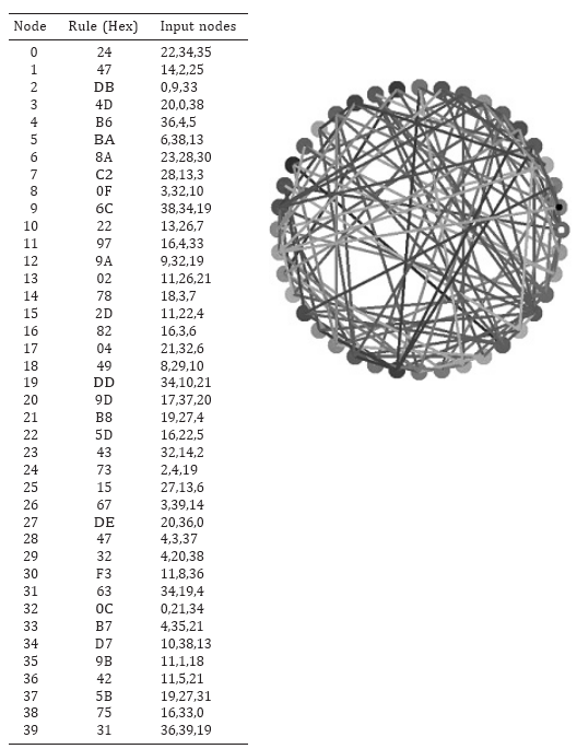
Fig. 1. An example of an N = 40, k = 3 Boolean network.
As no signal can pass a frozen node then it is not necessary to include those structural P-loops that contain frozen nodes when trying to determine the phase space p-loops. As we are only concerned with the asymptotic behavior of Boolean networks here, we can remove the frozen nodes of any particular network from the definition of that particular network.
Figure 2 shows a space–time diagram of one of the attractors (p12) for the network described in Fig. 1. It is clear that there are a number of frozen nodes that are directly responsible for restricting the potentially (quasi-) chaotic dynamics within a well-defined attractor basin. In this particular example, the nodes that are frozen are shown in Table 1. Bagley and Glass [1] refer to this as the attractor schema.
If the frozen nodes found for p12 were frozen for all attractors in the network of interest then the reduction process would already be nearly complete. However, this is often not the case. A trivial example would be for a network that contains a p1 attractor. For p1 attractors, all the nodes are frozen, and yet there may be other attractors in the system’s state space for which not all the nodes are frozen. If all the nodes really were frozen then the system could be reduced to a single point with one (structural) P1 loop. Of course, some networks do indeed converge on a single (state space) p1 attractor, but there are many systems that converge on a large number of different attractors, only one, or a portion, of which could be a p1. So as to not over-estimate the number of frozen nodes for the purposes of network simplification we must compare the set of frozen nodes for a subset of the full attractor set. By doing so we obtain the minimum set of frozen nodes, or the minimum attractor schema, and it is this set that is used to simplify the network’s P-structure. As we shall discuss later in this paper, these two are not always the same as the determination of the minimum set of frozen nodes can lead to an overestimation of the relevant elements.
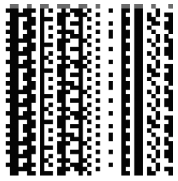
Fig. 2. Space–time diagram of the p12 attractor found via random sampling method for the network described in Fig. 1.
| Frozen Nodes | 0 | 3 | 7 | 8 | 9 | 10 | 12 | 13 | 14 | 16 | 17 | 19 | 22 | 26 | 28 | 31 | 32 | 34 | 37 | 38 |
| Frozen State | 0 | 0 | 0 | 1 | 1 | 0 | 1 | 0 | 0 | 0 | 0 | 0 | 1 | 1 | 0 | 1 | 0 | 1 | 1 | 1 |
Table 1. The frozen nodes of the p12 attractor found via random sampling method for the network described in Fig. 1.
By using the random sampling method described above, a subset of the full attractor set is easily found. It has already been suggested that the random sampling method can overlook some p-space structures (attractors) and so is not completely reliable. The difference here is that we are looking for the minimum set of frozen nodes, not the full set of phase space attractors. We will come back to the importance of this difference in a later section.
By starting with just 5,000 randomly selected initial conditions, five attractors (3p2, 1p12, 1p22) were found. The set of frozen nodes was found for each of these attractors. These sets were then compared and a set formed of those frozen nodes that were common in all those starting sets. Table 2 lists the set of frozen nodes for each of the five attractors found and is used to construct the minimum set of frozen nodes, which is assumed to contain all the frozen elements, no more no less. It is found that the minimum set of frozen nodes for this particular example contains a total of 21 nodes. The first step in simplifying the example network is to remove all reference to these particular nodes in the network description given
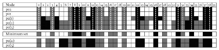
Table 2. The set of frozen nodes for each attractor found using the random sampling method with 5,000 samplings, and the construction of the minimum set of frozen nodes for this particular network. Nodes frozen to 1 are shaded black and those frozen to 0 are shaded dark grey. Note that the minimum set contains only those frozen nodes that are frozen to the same value whatever attractor they are on. Other frozen nodes can take on different freeze values depending on what attractor basin they are in, and some may actually be active rather than frozen. The p2(4) and p2(5) attractors were not found using the random sampling method but were found with a direct (full enumeration) method after the network was reduced.
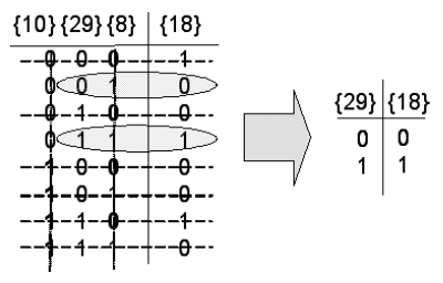
Fig. 3. The reduction of rule [&49] to rule [&2] for node {18}.
in Fig. 1. However, in removing these nodes the rules for the remaining nodes may now be incorrect and need simplifying themselves.
Rule Reduction
The inputs to node {18} in the example network and its corresponding Boolean function are {8, 29, 10}:[&49]. However, in the simplified version of this particular network, nodes {8} and {10} have been removed and so the functional rule [&49] is now incorrect. Correcting the rule is a straightforward matter and is shown in Fig. 3.
To do the rule simplification, we first note that {8} freezes to state 1 and {10} freezes to state 0. To correct and simplify the Boolean function, we simply remove any input configurations that correspond {8} = 0 or {10} = 1 (the reverse of the frozen states). By going through this process, the definition of node {18} becomes {29}:[&2].
This simple process is applied to all the remaining nodes in the reduced network.
Leaf Removal
Nodes that contain incoming connections, but that do not have any outgoing connections (outdegree = 0), contribute nothing to the qualitative structure of p-space. As such they can also be removed from the description of the network. No rules need to be adjusted as no other nodes depended on the state of these leaf nodes.
By applying the process described above, the original N = 40 network can be reduced to an N = 18 network that has exactly the same attractor set as the original network. The nodes that remain after this reduction process has been applied are referred to as the relevant nodes [4]. Figure 4 describes the reduced network. Now that the size of the network has been reduced from an unmanageable (in terms of applying a direct — full enumeration — method for determining state space structures) N = 40 to a manageable N = 18, we can easily run the network forward to fully enumerate the set of attractors that characterize this network’s p-space. As we are interested in finding the complete set of attractors rather than just one particular attractor, the backward pre-imaging approach described by Wuensche and Lesser [24] was not used. A simpler forward running method was used. This method simply starts with each possible state configuration and steps the network forward one time step. The step that was started with is then a pre-image for the state found after one time step. In this way, the pre-images of all the states in state space are found relatively quickly. Once the pre-images are found, we again start with the first state (in this case 000000000000000000) and run the network forward until an attractor cycle is found. Once found the entire attractor basin is constructed from the pre-image data. As each state is located on the attractor basin, it is removed from the list of potential starting states. The process is run through again by starting with the next state that has not yet been used as a starting condition. In this way, all the attractors are found without the repeated attempts that would undoubtedly occur if using a random sampling approach, and without the chance of missing out smaller attractor basins. However, whereas the random sampling approach is useful for larger networks, this more accurate direct method is only possible with networks smaller than ~25. As the network of interest here is only of size N = 18 then the more efficient and completely accurate approach is perfectly appropriate and practical.
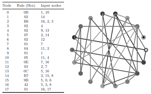
Fig. 4. A simplified version of the network shown in Fig. 1.
The result of applying this direct method is that the network of interest is actually characterized by a total of seven attractors (see Fig. 5), not five as was originally found using a random sampling method. The actual attractor set of the example network is 5p2, 1p12, 1p22 and not 3p2, 1p12, 1p22. The reason the additional two p2 attractors were not found using the random sampling method is that they are very small in comparison to the whole state space. Both attractor basins only contain 30 states each of which are organized in 8 clusters containing 3 or 6 states. Assuming the size of these attractors relative to the total number of states is the same in the full N = 40 network then the probability of finding one of the two is ~0.00003, or 1 in nearly 33,000. It is perhaps a little surprising that these two attractors slipped by unnoticed by the random sampling method of 100,000 samplings. However, ten repetitions of the random sampling approach with 100,000 sampling were performed and still neither of these two small basins was found. This suggests that the relative size (weight) of these two attractors is not the same in the full and reduced networks. Initial research (not reported here) confirms that there can be considerable differences between the relative weightings of attractor basins in the unreduced and reduced network forms (especially when Nreduced ≪ Nunreduced).
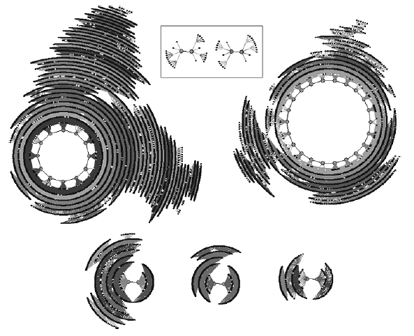
Fig. 5. The phase space of the reduced network. The phase space contains seven attractors: 1. p12, 91.52% (relative size of basin), &2D2A4 (state on attractor); 2. p22, 6.049%, &29292; 3. p2, 1.424%, &4D47; 4. p2, 0.703%, &24D47; 5. p2, 0.276%, &BAB5; 6. p2, 0.011%, &28F79, 7. p2, 0.011%, &292BC. The two small attractors in the box are the two that were not found after 100,000 random samplings of the original N = 40 network shown in Fig. 1.
What is also of note is that by applying the random sampling method again on the simplified version of the network of interest, with the same number of samplings (100,000), both of the previously missing p2 attractors were found. This is because the ratio of samplings to total number of states has hugely increased. Even if the network is not reduced to such a size that allows the application of a direct method, the random sampling method can be improved for a particular sampling rate by even a one-node simplification because as each node is removed, the size of state space is halved. This improvement is explored numerically in a following section.
Comparison with Random Sampling Method
Given that the frozen-node method described herein relies heavily on the random sampling method to find the minimum set of frozen nodes, it is necessary to examine how the frozen-node method is better. The problem with the random sampling method is that it can overlook small attractors even with relatively high sampling rates. To perform the frozen-node reduction method, we need not find the smallest attractor, but the minimum set of frozen nodes. However, there is a snag. If only a subset of the full set of attractors is used to determine the minimum set of frozen nodes, there is always the possibility that another attractor exists that contains a set of frozen nodes that would lead to a different determination of the minimum set. So in the absence of knowledge of all the attractors, there is the chance of over-determining the minimum set of frozen nodes, and thus over-estimating the relevant elements. (Of course, under-estimating them is not a problem unless we are particularly interested in knowing the reduced form accurately and not just a full qualitative characterization of phase space.)
To compare the relative error rates of the two techniques, the following experiment was performed. Firstly, the minimum set of frozen nodes and the attractor set were fully enumerated for a particular random Boolean network (for N = 15, k = 2) using the direct method described above. Then the minimum set of frozen nodes and the attractor set for the same network were again determined, but using the random sampling approach with varying numbers of samples (from 1 to 16,384). The results of the two approaches were then compared to see if there was an agreement in either the determination of the minimum set of frozen nodes and/or the attractor set. As one would expect, if the attractors sets agreed then so did the minimum set of frozen nodes. However, there were many instances where the reverse was not true, i.e., although the attractor sets found by the two methods differed; the determination of the minimum set of frozen nodes was in agreement.
This process was repeated for different sampling rates, each with 5,000 different random networks. The results are presented in Figs. 6(a) and (b) for N = 15, k = 2, 3, 4. The results clearly show that by using the random sampling, the chance of determining the minimum set of frozen nodes is considerably higher than determining the complete attractor set. For the case of N = 15, k = 2 the peak difference of 30% is found around a sampling rate of 0.00024%, which converts into only 8 random samples (out of a possible 215). The difference becomes more pronounced as k increases to 3 and 4. As we would expect, the difference tails off to zero as the number of samples tends towards the total number of states in state space. In the other direction, the difference tends to 20% as the sample size tends to 1. All in all, it is always easier to find the minimum set of frozen nodes than it is to find the complete set of attractors.
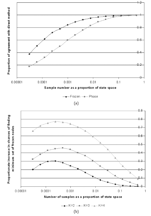
Fig. 6. (a) A plot showing the chances of finding the minimum set of frozen nodes (“Frozen”) and the attractor set (“Phase”) as a function of number of samples for N = 15, k = 2. (b) A plot showing the difference between “Frozen” and “Phase” for N = 15, k = 2, 3, 4.
The implications of this error analysis are that if the minimum set of frozen nodes is indeed found using the random sampling method (which is very much more likely than finding the full attractor set via the same means), then we have the chance of completely and without uncertainty finding the attractor set of a particular network. However, just because the minimum set of frozen nodes is always easier to find than the full attractor set, it does not necessarily follow that additional attractors are always found. One way to quantify the affect of the relative ease of finding the minimum set is to consider an ensemble of networks and count the number of attractors found using the simple random sampling technique, and the reduction technique discussed above.
In this experiment, the number of attractors for a particular network was determined using the random sampling method with varying sampling rates (1–8192). The minimum set of frozen nodes, which was identified using the attractors found via the random sampling method, was then used to find the reduced form of that particular network (both frozen nodes and leaves were removed and the functional rules adjusted). For the same sampling rate, the random sampling method was applied to the reduced form and the different attractors were counted. If the attractors found using this reduction method were found to be valid for the unreduced network (which is achieved by reconstructing the unreduced state from the reduced state using the frozen node data, and then running the unreduced network forward to confirm the presence of the expected p-loop), then these attractors were added to the cumulative count. If any of the attractors found in the reduced form were not found to be valid for the unreduced form (in which case the reduced form had not been found) then only the attractors found using the random sampling method on the unreduced form were added to the cumulative count. This process was repeated for 5,000 networks and for N = 10, 20, 40 and 60.
As the combined approach of random sampling → network reduction → random sampling requires approximately twice as much computing time as the simple random sampling approach then it needs to be demonstrated that the combined approach finds more attractors than running the simple random sampling approach with twice the sampling rate. (Note: it is actually not quite twice the amount because of the additional reduction steps, but these are relatively insignificant when compared to the computer time needed to run the random sampling step twice. Furthermore, the second random sampling step is performed on the reduced network which in most cases is smaller than the unreduced network — except in the cases of irreducible networks — and therefore less computer time is needed to perform this secondary step. As an over-estimated approximation, it will be assumed that twice the computer time is needed.) Figure 7 shows the cumulative attractor count for both the simple random sampling approach and the combined approached for a range of sampling rates. Figure 8 plots the difference (as a percentage) between the two approaches.
Figures 7 and 8 clearly illustrate that above a certain sampling rate the combined method (random sampling → network reduction → random sampling) is rather more efficient than the simple random sampling approach. For example, if we consider the case for N = 60: at a sampling rate of 5.55 × 10⁻¹⁷ samples per state (S(1/N) - 1 = 0.07, or 64 samples) 31,558 attractors are found in total (for the 5,000 networks considered). This is 25.9% greater than the number of attractors found using the simple random sampling approach with the same sampling rate. To find 31,558 attractors using the simple random sampling approach, a sampling rate of slight less than 4.4 × 10⁻¹⁶ is needed. This is about 8 times the sampling rate used for the combined approach clearly showing the benefits of utilizing the combined approach when counting attractors for a network ensemble. In the case of N = 60, a sampling rate of 2.22 × 10⁻¹⁶ samples per state (S(1/N) - 1 = 0.10, or 256 samples) corresponds with a total of 42,171 attractors. The simple random sampling approach only finds only 39,112 attractors (~7% lower) with a sampling rate 32 times greater than the combined approach! The data for N = 10 shows that, although the combined approach is more efficient, after some point (as we get closer to the true number of attractors and as the number of samples tends towards the number of states) diminishing returns are realized with increasing computing time (as we would expect).
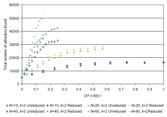
Fig. 7. A plot comparing the two attractor counting approaches: (1) random sampling (Approx) and (2) combined random sampling → network reduction → random sampling (Reduced).
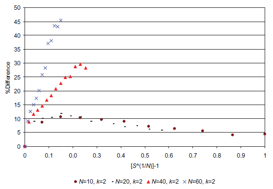
Fig. 8. A plot showing the percentage increase in attractors found by using the combined method, combined random sampling → network reduction → random sampling. We would expect all curves to have a similar profile as the N = 10 curve. Also note that if the sample states that were tried were stored so that they would not be generated again then the curves would all tend to 0 as S(1/N) - 1 tended to 1.
Summary and Conclusions
It has been shown that the removal of frozen nodes and leaf nodes can be used to simplify the compositional complexity of random (synchronous) Boolean networks. The approach described is not foolproof (although it is a trivial matter to check whether or not the additional attractors found are valid), but it does offer a greater chance of determining the attractor set of larger Boolean networks than using a simple random sampling method only. Given the relative ease by which this method can be incorporated into simulation-based analyses of Boolean networks, the fact that the occurrence of arbitrarily small attractor basins increases with network size, and that often simulation methods are the only way to validate analytical studies, it is suggested that this simplification step be included in any simulation-based analysis of synchronous random Boolean networks. Indeed, the evidence presented in the previous section clearly shows the computational savings in utilizing this particular method. Even though the chances of failing to find all attractors increases with network size, the combined approach discussed herein certainly improves our chances of finding a larger subset of attractors, if not the complete set.
Bastolla and Parisi [5] showed that Boolean networks spontaneously organize themselves into dynamically disconnected modules. A further improvement to the method presented herein may be to identify the modules in the reduced networks and then use the random sampling method to find the attractors for each module. It is then a straightforward matter to find the attractors for the composite network as the modules are dynamically disconnected. This additional step may prove most useful in the frozen and critical phases as the majority of networks in the chaotic phase contain only a single module. Further studies are required to confirm whether or not the improved accuracy in counting attractors is justified given the additional computational time needed to identify network modules.
There are at least two broader issues that the research reported herein can contribute to the discussion of. The motivation for the research that lead to this paper came from a statement by Cilliers [8] that one of the traits of complex systems is that they are incompressible, or irreducible. Clearly, the simplification described herein does result in loss of detail. For starters, we are only concerned with the qualitative aspects of state space, and therefore a lot of quantitative (transient) detail is lost. In this sense, the networks really are irreducible. However, it is equally clear that if we relax our need for complete detail, reduction methods can lead to useful and robust qualitative understanding. Complex systems may well be incompressible in an absolute sense, but many of them are at least quasi-reducible in a variety of ways. This fact indicates that the many commentators suggesting that reductionist methods are in some way anti-complexity — some even go so far as to suggest that traditional scientific methods have no role in facilitating the understanding of complexity — are overstating their position. Often linear methods are assessed in much the same way. The more modest middle ground is that though complex systems may indeed be incompressible, many, if not all, methods are capable of shedding some light on certain aspects of their behavior. It is not that the incompressibility of complex systems prevents understanding, and that all methods that do not capture complexity completely are useless, but that we need to develop an awareness of how our methods limit our potential understanding of such systems. In this paper, we have limited ourselves to a concern with the qualitative asymptotic behavior of selected complex systems and have described a method that delivers a way of obtaining that understanding. In a sense, complexity has been compressed, but there are many routes to the simplification of complexity, each leading to perfectly valid, albeit limited, understanding.
Acknowledgments
The author would like to thank Michael Lissack and his foundation for supporting the research reported herein — few institutions afford such intellectual freedom. He is also appreciative of two anonymous reviewers for useful comments and suggestions that encouraged performing further experiments to support the argument presented, and helped avoid at least one silly mistake! As always thanks also goes to Caroline, Alexander and Albert for interesting diversions.
References
[1] Bagley, R. J. and Glass, L., Counting and classifying attractors in high dimensional dynamical systems, J. Theor. Biol. 183, 269–284 (1996).
[2] Bastolla, U. and Parisi, G., Closing probabilities in the Kauffman model: An annealed computation, Physica D 98, 1–25 (1996).
[3] Bastolla, U. and Parisi, G., Attraction basins in discretized maps, J. Phys. A: Math. Gen. 30, 3757–3769 (1997).
[4] Bastolla, U. and Parisi, G., Relevant elements, magnetization and dynamical properties in Kauffman networks: A numerical study, Physica D 115, 203–218 (1998).
[5] Bastolla, U. and Parisi, G., The modular structure of Kauffman networks, Physica D 115, 219–233 (1998).
[6] Bilke, S. and Sjunnesson, F., Stability of the Kauffman model, Phys. Rev. E 65, 016129 (2002).
[7] Chowdhury, D. and Stau?er, D., A generalized spin model of financial markets, Eur. Phys. J. B8(3), 477–482 (1999).
[8] Cilliers, P., Complexity and Postmodernism (Routledge, 1998).
[9] Derrida, B. and Weisbuch, G., Evolution of overlaps between configuration in random networks, J. Phys. Paris 47(8), 1297–1303 (1986).
[10] Derrida, B., Dynamics of automata, spin glasses, and neural networks, Notes for School at Nota, Sicily; Valleys and overalps in Kauffman’s model, Phil. Mag. 56, 917–923 (1987).
[11] Derrida, B. and Flyvbjerg, H., Multivalley structure in Kauffman’s model: Analogy with spin glasses, J. Phys. A: Math. Gen. 19, L1003–L1008 (1986).
[12] Dunne, P., The Complexity of Boolean Networks (Academic Press, CA, 1988).
[13] Garson, J. W., Chaotic emergence and the language of thought, Philos. Psychol. 11(3), 303–315 (1998).
[14] Horgan, T. and Tienson, J., A nonclassical framework for cognitive science, Synthese 101(3), 305–345 (1994).
[15] Jacob, F. and Monod, J., On the regulation of gene activity, in Cold Spring Harbor Symp. Quantitative Biology (26) (Cold Spring Harbor, NY, 1961), pp. 193–211.
[16] Kauffman, S. A., Metabolic stability and epigenesist in randomly connected nets, J. Theor. Biol. 22, 437–467 (1969).
[17] Kauffman, S. A., Emergent properties in random complex automata, Physica D 10, 145 (1984).
[18] Kauffman, S. A., The Origins of Order: Self-Organization and Selection in Evolution (Oxford University Press, NY, 1993).
[19] Kauffman, S. A., The At Home in the Universe: The Search for Laws of Self- Organization and Complexity (Oxford University Press, Oxford, 1995).
[20] Khalil, E. L., Nonlinear thermodynamics and social science modeling: Fad cycles, cultural-development, and identification slips, Am. J. Econ. Sociol. 54(4), 423–438 (1995).
[21] Stern, M. D., Emergence of homeostasis and ‘noise imprinting’ in an evolution model, Proc. Nat. Acad. Sci. 96, 10746–10751 (1999).
[22] Tocci, R. J. and Widmer, R. S., Digital Systems: Principles and Applications, 8th edn. (Prentice Hall, NJ, 2001).
[23] Weigel, D. and Murray, C., The paradox of stability and change in relationships: What does chaos theory offer for the study of romantic relationships?, J. Soc. Pers. Relat. 17(3), 425–449 (2000).
[24] Wuensche, A. and Lesser, M., The Global Dynamics of Cellular Automata: An Atlas of Basin of Attraction Fields of One-Dimensional Cellular Automata, 2nd edn. (Discrete Dynamics Inc., Santa Fe, NM, 2000).