Introduction
Social networks are complex systems that are characterized by high numbers of interconnected component entities, and a high degree of interaction between these entities. The interrelationships in such a network are dynamic and evolve over time. Temporal changes in social networks are difficult to understand and anticipate. The interrelationships between the component entities in a social network and its global behavior can be so numerous and mostly hidden, and can affect so many different entities throughout the social network that it becomes extremely difficult to comprehend.
Complexity theory is ideally suited to study social networks. Complex adaptive systems theory is a branch of complexity theory that studies systems that consist of agents that are collectively able to evolve in response to environmental changes. The agents in such a system constantly act and react to the actions of other agents and events in the environment. A social network is a complex adaptive system, in which people are agents interacting with each other.
In order to understand social complexity, the local behaviors of the participants must be understood, as well as how they act together and interact with the environment to form the whole. To model this, we use Bayesian network techniques to mine and model emergent relationships between local behaviors and global behaviors in social networks over time.
Social Complexity
The complex structure of any social organization can be thought of as a network of individuals/agents (Nohria & Eccles, 1992: 288; Lincoln, 1982), sometimes termed network actors, that operates and is operated on in an environment which itself is an environment of other distributed organizations (Van Wijk et al., 2003; Potgieter et al., 2006), and the actions of agents within the network are shaped and constrained because of their position and embeddedness in the network (Nohria, 1992).
Complex adaptive systems theory, a branch of complexity theory that is well suited to study social networks, investigates systems that consist of agents that are collectively able to evolve in response to environmental changes (i.e., people who interact with each other in socially complex ways). Social networks are complex systems that are characterized by high numbers of dynamically interconnected component entities, and a high degree of time-based evolutionary interactions between these entities. Temporal changes in social networks are difficult to understand and anticipate, because of the structures of constraint and opportunity negotiated and reinforced between interacting individuals. The interrelationships between the component entities in a social network and its global behavior can be so numerous and mostly hidden, and can affect so many different entities throughout the social network that it becomes extremely difficult to comprehend. Such changes, for modern organizations, can come in the form of globalization, deregulation, competition, technology and political transformation. The agents in such a constantly changing system tend to step out of the traditional boundaries of their network (within-group identification), act and react to, and evolve in relation to, the actions of other agents and events in the environment to achieve a more desirable end, e.g., to learn faster in the changing environment, or to collaborate better, or to craft more relevant identities, or to seek help in making major decisions, or to negotiate and renegotiate relationships of power, etc.
In social network studies, the traditional archetype—which acts as an interpretive schema—of an organization is that it is made up of a number of static departments, which themselves have specialised individuals (agents), and its strategy for competing, or winning, or succeeding, or sustaining itself is fixed for a time period, usually 1-3 years, and is clearly understood and acted upon by its agents. After the specified period, usually the organizational strategy is reviewed, altered, or rewritten or totally revoked in favour of a new strategy, and its agents then enact new behaviors against such a plan. We contend, however, that organizations are not static, atomistic agents, instead they are recurring in dynamic agent linkages and embedded in networks of increasing importance (Brock, 2006) that progressively influence competitive actions (Granovetter, 1985, 1992; Burt, 1995) and may themselves challenge the interpretive schema and supportive structures, and ultimately even delegitimize the existing archetype.
Social Network Analysis and Link Prediction
Social Network Analysis (SNA) is a research area aimed at understanding social complexity by representing and analyzing social networks using mathematical graphs. This was first done by researchers, such as Cartwright and Harary (1956) in the USA, who interpreted Kurt Lewin’s social interaction theory into graph theory—thereby helping to transform the study of social networks from description to analysis. In this theory, a graph G is a structure consisting of a set of nodes V (also called vertices), and a set of links E (also called arcs or edges). In our discussion the terms graph, network, social network and sociogram are used interchangeably. A graph can be bi-directed1, meaning that we are not concerned about the order of the nodes in a link. Alternatively, a graph is directed, meaning that the nodes in a link form an ordered pair. Nodes represent people and links represent some type of relationship between people. For the purposes of this discussion a link exists between two people if they have exchanged a message in the past. Thus links are never removed once they have been formed.
There appears to be one standard textbook on SNA (Wassermann & Faust, 1994), cited by the large majority of researchers in this field. Although SNA has existed for over fifty years, most analysis techniques have been designed for static data, or at least a static archetype of social organization. For example, Wassermann and Faust (1994) contains no mention of temporal metrics, even though it was written in 1994 when electronic networks were well established. With the increase in the use of computers, collecting enough data to create numerous graphs over fixed time intervals becomes possible. An example is creating a graph per week from email data, using a server’s email log of ‘to’, ‘from’, and ‘date’ fields (Campbell et al., 2003). This series of graphs can be used to study the evolution of the network and the change over time in various metrics. Predicting certain changes to a social network is called the link prediction problem. Liben-Nowell and Kleinberg (2003) explain it as:
Given a snapshot of a social network at time t, we seek to accurately predict the edges that will be added to the network during the interval from time t to a given future time t’.
Link prediction has many real world applications, especially in the fields of marketing and crime prevention. Examples include:
Identifying the structure of a criminal network (i.e., predicting missing links in a criminal network using incomplete data).
Overcoming the data-sparsity problem in recommender systems using collaborative filtering (Huang et al., 2005).
Accelerating a mutually beneficial professional- or academic connection that would have taken longer to form serendipitously (Farrell et al., 2005).
Improving hypertext analysis for information retrieval and search engines (Henziger, 2000).
Monitoring and controlling computer viruses that use email as a vector (Lim et al., 2005).
Predicting when webpage users will next visit, in order to improve the efficiency and effectiveness of a site’s navigation (Zhu, 2003).
Link prediction might also be useful in ecology, though interdisciplinary sharing between these two fields is still new (McMahon et al., 2001).
Metrics
Link prediction through topological analysis is performed by computing various metrics. A metric is a value calculated from a graph that describes the graph in some way. For instance, it is more likely that two nodes that both have a high degree (number of neighbours) are more likely to form a new link, than two nodes with a low degree (Liben-Nowell, 2005). Most traditional SNA metrics are described and defined in Wassermann and Faust (1994), and summarised in an online book by Hanneman (2001). We defined metrics to quantify local behaviors of agent resources in social resource combinations (Potgieter et al., 2006). The appearance of new links between individual agent resources is emergent behavior of the social network. Table 1 lists the metrics that were used for link prediction in this research. They were chosen since prior research has found them to be useful. Huang et al. (2005) found that the most useful dyadic metrics for link prediction, in descending order, were the Katz measure, preferential attachment, common neighbours and the AdamicAdar number. Recency is a metric that, to the authors’ knowledge, has not been used before. The table uses certain symbols that are now defined:
# denotes the number of elements in a set. Un is the set of bi-directed links of the social network at time step n. A bi-directed link between nodes vi and vj is notated as ui,j and uj,i. ?(vi) is the set of neighbours of node vi, i.e., the set {vj: ui,j ? U}.
P(vi, vj) is the set of all shortest paths from vi to vj. P(vi, vj, vx) is the set of all shortest paths from vi to vj that pass through node vx.
Existing link prediction techniques use the values of metrics in a graph to determine where new links are likely to arise. Important contributions to the field include Popescul and
Ungar (2003), Taskar et al. (2004), Popescul and Ungar (2004), and Zhou and Scholkopf (2004). The classic paper on link prediction is by Liben-Nowell and Kleinberg (2003). They tested the predictive power of only proximity metrics, including common neighbors, the Katz measure and variants of PageRank. They found some of these measures had a predictive accuracy of up to 16% (compared to a random prediction’s accuracy of less than a percent). A third of Liben-Nowell’s doctoral thesis (Liben-Nowell, 2005) was a chapter on link prediction in social networks. A few other link prediction papers are summarized in Getoor and Diehl (2005).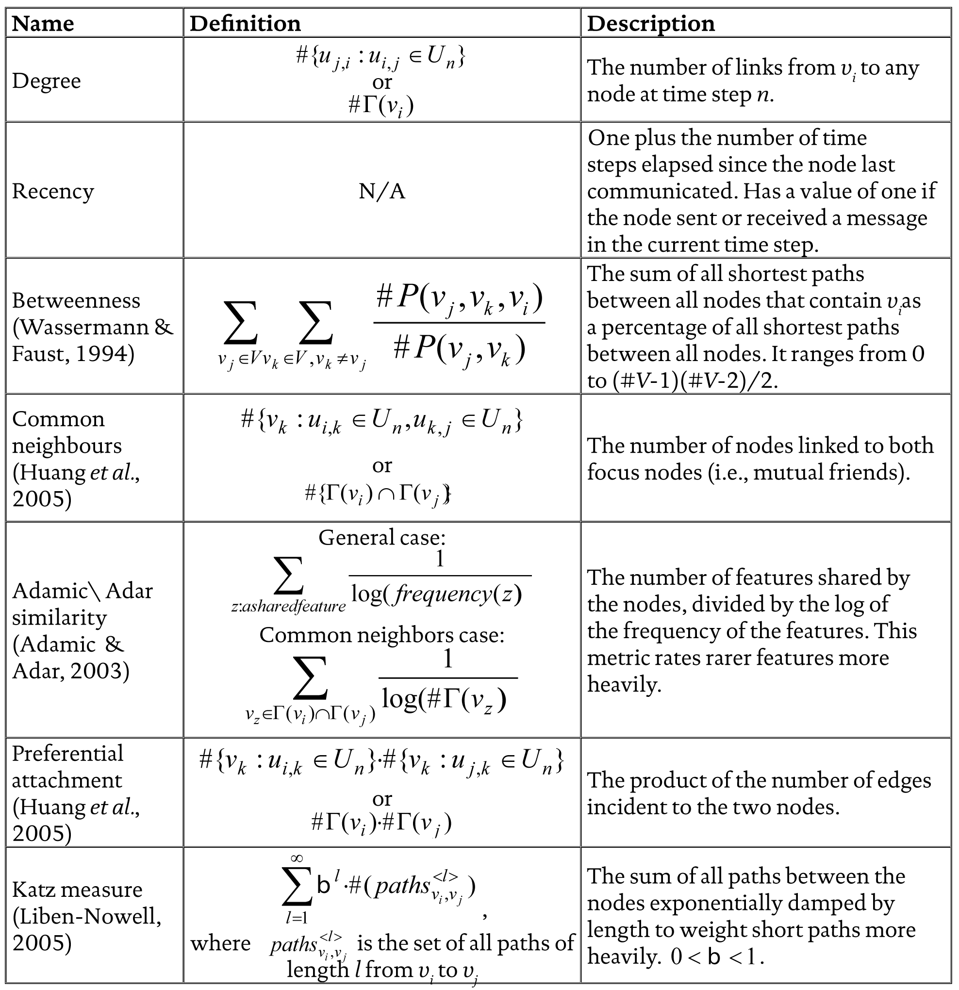
Past Contributions to Temporal Analysis
Leskovec et al. (2005) state that little work has been done on analyzing long-term graph trends:
Many studies have discovered patterns in static graphs, identifying properties in a single snapshot of a large network, or in a very small number of snapshots; these include heavy tails for in- and out-degree distributions, communities, small-world phenomena, and others. However, given the lack of information about network evolution over long periods, it has been hard to convert these findings into statements about trends over time.
Their study of trends found that, over time, graphs densify and the average distance between nodes decreases. This was contrary to the existing beliefs that the average nodal degree remains constant and average distance slowly increases. They claimed that existing graph generation models are not realistic and proposed a new “forest-fire” generation model. Desikan and Srivastava (2004) studied the change in metrics of a set of webpages over time for the graph as a whole, and for single nodes (subgraphs are their current research). They found that temporal metrics, such as their Page Usage Popularity, can be effectively used to boost ranks of recently popular pages to those that are more obsolete. This seems to indicate that temporal metrics are a useful addition to traditional static metrics in the study of some networks.
Using Temporal Analysis to Aid Link Prediction
To date no temporal information has been used in link prediction research (excluding our earlier proposition of the idea in April et al. (2005) and Potgieter et al. (2006). It is the authors’ opinion that ignoring such information excludes valuable temporal trends that emerge in sociogram sequences that may greatly increase the accuracy of link prediction. We have three types of temporal metrics that have been defined, the first two of which are borrowed from finance:
Return is the percentage increase or decrease of a value over a period of time (Ross et al., 2001). It shows the rate of change of a given metric. For instance, if we are considering the degree of node vi from time step one to time step fifty, the degree return would be:
Moving averages are used to extract long-term trends from short-term noise. They do not show trends or “movement”, like return, but rather serve only to blur the values of the metrics around a point;
Recency (Table 1), simply shows how much time has elapsed since a node has communicated.
Temporal Analysis Methodology
All the metrics listed in the Table 1 were calculated for a series of hundred networks constructed daily from information extracted from the Pussokram online dating network dataset. In addition to the computation standard metrics, their moving averages over twenty, ten and two days were computed, as well as their returns over the same period and the recency of each node. Up to one hundred sample dyads where new links formed on the day, and an equivalent number of unconnected dyads, were chosen for each network. There were 9,939 cases of each class in total. Logistic regression (Hosmer & Lemeshow, 1989) in the Weka data mining system (Witten & Frank, 2005) was used to perform link prediction. The dataset was split into a 70%/30% train/test division, and after the system was trained it predicted whether a given set of test instance metrics characterized a forming link or an unconnected link. The overall classification accuracy, the true positive rates for each class, and the kappa statistic (a measure of a system’s accuracy improvement over a random guess) were calculated (Witten & Frank, 2005). The true positive rate of a class is the percentage of all the instances of that class that were predicted correctly. The kappa statistic is defined as:
where P(A) is the total percentage accuracy of instances predicted by the learning system and P(E) is the total percentage accuracy of instances predicted by random guessing. Since in this research an equal number of positive and negative instances were used we know that P(E) = 0.5 and 1-P(E) = 0.5, which we applied to the kappa statistic. A kappa value over 0.4 has been said to indicate ‘good agreement beyond chance’ (Fleiss, 1981).Temporal Analysis Results and Conclusions
Table 2 shows the mean and standard deviation for each class, as well as the significance level of the mean difference using a Normal statistical difference of means test. The last column is the most important and shows the kappa value of each metric when used alone in a logistic regression against the class. The suffix ‘F’ stands for ‘From’ (the first node in a dyad instance), the suffix ‘T’ stands for ‘To’ (the second node in a dyad instance). ‘A’ stands for ‘Average’, ‘R’ stands for ‘return’ and the numbers ‘20’, ‘10’ and ‘2’ stand for the number of time steps over which the average and return were calculated. The metric in the middle row of each group is the traditional static metric. The averages are shown above it and the returns are shown below. ‘Forming’ and ‘Unconnected’ are emergent properties of the social network. Forming means that a link does not exist in the current time step, but it will appear in the next time step. Unconnected means that link between two nodes does not exist in the current time step, and these nodes will remain unconnected in the next time step.
We can see that almost all metrics had significant differences between each class. Thus the significance levels become meaningless and we consider only the kappa statistic as a measure of worth. A kappa statistic of 40% corresponds roughly to an overall accuracy of 70%, and a kappa of 20% corresponds to an accuracy of 60%. We note that a metric’s moving average is a better link predictor than the static metric (except in the case of recency, which is already a temporal metric). Furthermore, the increase in predictive accuracy of moving averages seems to level off somewhere between ten and twenty time steps prior to the current time step. Thus, it is recommended that taking averages further back than twenty time steps is unnecessary and extravagant. Finally, metric returns appear to be completely useless for link prediction and should not be used in the future.
Table 3 shows how the metrics perform in combination to predict links. This is the ultimate test of prediction accuracy—seeing how well we can classify links as forming or not (global behaviors) using any combination of metrics (local behaviors) at our disposal.
The first row shows the accuracy of static metrics alone. The second row shows the accuracy of the same metrics using moving averages. It can be seen that the overall accuracy increases by 6% from the first row to the second. If we include the recency metrics as well the accuracy increases to 82%, with true positive rates above 80% for both classes. This shows that temporal metrics are an extremely valuable new contribution to link prediction and should be used in future applications. Further research to be performed includes suggesting new temporal variations of static metrics and determining exactly the optimum number of time steps over which to compute temporal metrics.
Using Bayesian Networks to Understand Social Complexity
In order to understand social complexity, the local behaviors of the participants/network actors must be understood, as well as how they act together and interact with the environment to form the whole. To model this, we used Bayesian network techniques.
According to Baas and Emmeche (1997), understanding is related to the notion of explanation. A complex adaptive system uses the hyperstructures in its internal model for explanation and understanding. It uses observation mechanisms to create and maintain these hyperstructures. The process of adaptation relies heavily on the observation mechanisms and involves a progressive modification of the hyperstructures (Holland, 1995).
We measured local behaviors using metrics and we used Bayesian networks to model the interrelationships between the metrics as local behaviors and links forming between individuals as emergent behaviors. We also explored how the metrics evolve over time using Dynamic Bayesian Networks.
Table?2
Metric statistics, grouped by category
Table?3
Metric sets prediction
Link Prediction using a Bayesian Network
Bayesian Networks provide the ideal technology to reason about social resource combinations (Potgieter et al., 2006). A Bayesian network is a directed acyclic graph (DAG) that consists of a set of nodes that are linked together by directional links. Each node represents a random variable or uncertain quantity. Each variable has a finite set of mutually exclusive propositions, called states. The links represent informational or causal dependencies among the variables, where a parent node is the cause and a child node the effect. The dependencies are given in terms of conditional probabilities of states that a node can have, given the values of the parent nodes (Pearl, 1988). Each node has a conditional probability matrix to store these conditional probabilities, accumulated over time.
Bayesian learning can be described as ‘mining’ the structure of the network and calculating the conditional probability matrices from history data. The data may be incomplete and the structure of the Bayesian network can be unknown.
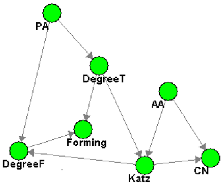
Figure 2 illustrates the Bayesian network that was mined from the same dataset used in the temporal analysis. It clearly illustrates the cause-effect relationships between the local behaviors (metrics ‘PA’, ‘DegreeT’, ‘DegreeF’, ‘Katz’, ‘AA’ and ‘CN’) and the emergent behavior ‘Forming’.
With a cross validation method, we extracted 30% records at random from the entire dataset of over 19,000 instances as used in the temporal analysis. The test set contained over 8, 000 records. The remaining 70% (over 11, 000) records served as the training set. As one of the pre-processing steps, we discretized the training and the test sets using the equal width algorithm (Osunmakinde, 2006). The pre-processed training set was used by the Hybrid Genetic Algorithm (Osunmakinde, 2006) to mine a Bayesian Network model, shown in Figure 2. This algorithm is described later in this paper.
After training, we used Bayesian Inference in the model in Figure 2 to classify the 30% test set. Bayesian inference is the process of calculating the posterior probability of a hypothesis H (involving a set of query variables) given some observed event (assignments of values to a set of evidence variables e), P(H|e).
For the link prediction, the hypothesis will be that ‘Forming’ is true or false, given the values of the evidence variables ‘DegreeT’, ‘DegreeF’, ‘Katz’, ‘PA’, ‘AA’, ‘CN’:
P(Forming = true | DegreeT, DegreeF, Katz, PA, AA, CN) ?
Or,
P(Forming = false | DegreeT, DegreeF, Katz, PA, AA, CN) ?
The confusion matrix (Ron & Foster, 1998) in Table 4 gives the link prediction and evaluation of the results. The implementation results were computed and generated from Table 4 and presented in Table 5.
Modelling Emergent Social Network Behavior over time using a DBN
A Dynamic Bayesian network (DBN) is ideally suited to model changes in metrics and emergent behavior over time. In Dynamic Bayesian networks, multiple copies of the variables are represented, one for each time step (Pearl & Russell, 2000). A DBN provides a compact representation of temporal probabilistic processes such as Hidden Markov Models (HMM). It contains slices of sub-models which facilitate its probabilistic reasoning over time. That is, we can interpret the present, understand the past and predict the future. We want to compute: P(Xi(t) | E(t1:tn)) from the
Table?4
Confusion Matrix
| Predicted values | ||
| Actual values | True | False |
| Forming = false(Total 4390) | 4390 | 0 |
| Forming = true(Total 4390) | 39 | 4351 |
Table?5
Implementation results
| True positive rate of forming | 99.1116173120729% |
| True positive rate of not forming (unconnected) | 100.0% |
| Kappa | 99.1116173120729% |
| The overall accuracy | 99.55580865603645% |
where (Xi(t)) represents the i'th hidden or unobservable variable at time t and E(t1:tn)) refers to the observable evidence from time step t1 to tn. Observe that this follows a Markov assumption where the current state depends on only finite history of previous states (Russell & Norvig, 2002).
The construction of the DBN requires the following information components:
The prior distribution over the state vari1. ables, P(X0);
The transition model, P(Xt | Xt-1), and;
The sensor model, P(Et|Xt).
The learning of these components depends on the topological connections between the successive slices, the hidden states and the evidence variables. There are many algorithms for learning parameters in DBNs. Where sufficient training data is available, a maximum likelihood estimate (MLE) can be used. Many areas of science and engineering use approximate inference algorithms in DBNs because of the shortcomings of exact inference (Pavlovic et al., 2001).
In this paper, we incorporate a Dynamic Bayesian Network illustrated in Figure 3 which models possible relationships between metrics and forming links. The observable nodes are ‘Forming’, ‘DegreeT’, ‘DegreeF’, ‘Katz’, ‘PA’, ‘CN’ and ‘AA’ which serve as the evidence variables ‘E’, to the unobservable variable called ‘HiddenNode’. We tested this DBN using the 150 time slices of the dataset used in the temporal analysis, using the metrics defined in the previous sections. The primary objective of this DBN is to predict relationships between metrics (local behaviors) and links forming (global behaviors) in future time steps. Using this, possible links can be predicted between two or more people using the predicted relationships from observed nodes.
Dynamic Bayesian Network Methodology
We used the same dataset as in the temporal metrics analysis, consisting of 150 time steps and used 70% as a training set, while 30% was used as a test set by a hybrid genetic algorithm (see next section). The average number of records in each time step was 201.
In our implementation, we trained the three components of DBN using the MLE (Russell & Norvig, 2002) and Mutual Information in information theory (Cheng et al., 1997). These 3 components were used during DBN inference using the Viterbi algorithm (see next section). We evaluated the relationships predicted by the DBN using the hybrid genetic algorithm. The DBN did not have access to the 30% dataset, but it was used by the genetic algorithm. That is, the genetic algorithm mined the actual relationships between the metrics and forming links at each time step, while the DBN predicted relationships between the metrics and forming links at each time step.
Dynamic Bayesian Network Prediction using the Viterbi Approximation
By definition (Pavlovic et al., 2001) the probability of the partial optimal path to a hidden state i at time t when evidence zt is observed implies:
?(i) = maxj(?t-1(j)ajibizt)
where ‘delta’ is the probability of reaching a particular intermediate hidden state on the DBN time slices, ‘a’ is the transition probability while ‘b’ is the corresponding observation probability. Recall the Markov assumption that says that the probability of a hidden state occurring, given the previous history, depends on the previous i-states. We wanted to compute the probability of the most probable path to any hidden node X. That is:
P(Xt) = Maxi P(it-1)P(X | a)P(observationt | X)
We used the knowledge of the previous states; the transition probabilities multiplied by the corresponding observation probabilities. This calculated the hidden node.
The HGA is a variant of classical genetic algorithm operators because it integrates information theoretic measures as learning components and mathematical concepts as
population construction. Specifically, some of the information theoretic measures we used were: Mutual Information (MI) model, Shannon’s information content, and Minimum Description Length (MDL) model. Also, the mathematical component part of the HGA was a PowerSet lattice which implemented crossover operator. Moreover, PowerSet lattice generated population space from which the best networks could emerge.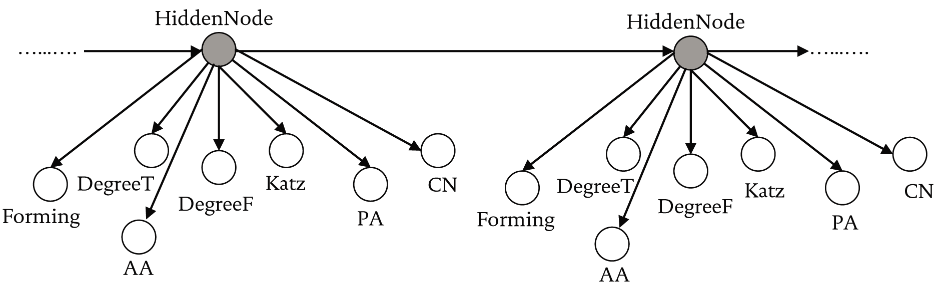
One of the interesting features of this methodology is that the components of the HGA were implemented as decomposable systems. The decomposability means the functionalities of every component such as MI perceives its inputs and produces its outputs differently from other HGA components. However, such decomposability of every HGA component is to level complexity into simplicity. More information can be found in Osunmakinde (2006).
Examples of the predicted relationships by the Dynamic Bayesian Network for time step 1 were as shown in Table 6.
We compared the relationships predicted by the DBN with the actual relationships mined using the hybrid genetic algorithm. We calculated the accuracy of each prediction by counting the number of predicted relationships and actual relationships that correspond in structure predicted by the DBN and the actual structure mined by the HGA. We obtained the results detailed in Table 7.
In future research, we will use these predicted relationships to study to see if time graphs densify over time and at what rate the average distance between nodes decreases.
Conclusion
In this paper, we recognise the role of complex adaptive systems theory in shedding light on an increasingly important aspect of organizational life (and survival), namely, social networks, and emergent temporal phenomena in these networks. It is our contention that the fluidity and temporality of the interrelationships, making up such networks, render it dependent on changing contexts—and therefore accurate prediction, going forward, becomes difficult (near impossible) using traditionally static methodologies.
The use of link prediction to improve collaborative filtering in recommender systems was investigated (Huang et al., 2005), and the Katz measure was found to be the most useful, followed by preferential attachment, common neighbors and the AdamicAdar measure. These path-based and neighbor-based measures outperformed simpler metrics, and so we used these in our experiments. We were able to show that when emergent temporal trends are ignored in sociogram sequences, the link prediction accuracy is significantly lower than when included.
Table?6
Relationships predicted by DBN
Table?7
DBN Prediction Accuracy
An important contribution of this paper is that we have shown that temporal metrics are an extremely valuable new contribution to link prediction, and should be used in future research and applications. This is significant because, to date, no temporal information has been used in link prediction research, excluding our earlier proposition of the idea in April et al. (2005) and Potgieter et al. (2006). Further research to be performed includes suggesting new temporal variations of static metrics and determining exactly the optimum number of time steps over which to compute temporal metrics.
We have used Bayesian networks for link prediction, and achieved extremely high prediction accuracies. Additionally, we trained the components of the Dynamic Bayesian Network in order to mine the actual relationships between the metrics (local behaviors) and forming links (emergent global behaviors) at each time step—of significance is the fact that the DBN was able to predict relationships between the metrics and forming links at each time step, as it evolved over time. In future research, we will use these predicted relationships to study more emergent temporal phenomena such as if time graphs densify over time and at what rate the average distance between nodes decreases.