Introduction
Utility–service provision is a process in which utility products such as water, electricity, food, etc. are delivered to households to satisfy basic human needs such as nutrition, adequate quantity and quality of water, thermal comfort, and wants such as leisure. These products can either be delivered via infrastructure or produced locally, e.g., electricity can be produced from sunlight using solar panels or water can be harvested from rainwater and subsequently treated to drinking water standards1.
Utility infrastructures such as power grids, water and gas pipelines, or transportation and communication systems can be considered as complex networks with similar topological and dynamic properties to the World Wide Web2 that additionally depend on the traffic and the pattern of connections. We can divide such complex networks into four categories, originally proposed by Newman3:
Social networks in which a set of people form patterns of contacts or interactions, e.g., friendships, thematic groups, mutual likes and hobbies, etc.;
Information networks, otherwise referred to as knowledge networks, e.g., the network of citations between academic papers or the World Wide Web where web pages are linked via hyperlinks pointing from one page to another;
Biological networks such as the food web, in which nodes represent species in an ecosystem and directed edges between two nodes indicate that the former species prays on the latter one4;
Technological networks designed for distribution of some commodity or resource, e.g., information, water, electricity, etc.; such networks are the main focus of this paper.
Utility–service provision can be considered as a technological network and analyzed as such since its main objective is to deliver different utility products to households and then convert these utility products using different devices into services in order to satisfy basic human needs and wants. This task is very complex as its success depends on multiple factors such as proper functioning of devices and the infrastructures delivering the required utility products. Failure of one or more of these components might possibly deprive the users of a product and thus, service, for an unknown amount of time.
The complexity utility–service provision becomes more visible when we look at the structure of a typical utility infrastructure which is hierarchical and can be divided into households, communities, districts and cities. A household is a component of a community, the community can be a part of a district in a city whilst cities can be regarded as hubs in a country-wide network. Each level of this hierarchy has its own structure and distinct operational properties. Such a hierarchical structure creates complexity as the behavior of the overall behavior of the cities and districts emerges from the combined behavior of single households. However, it is difficult to deduct the features of a city from the characteristics or properties of an individual households due to inherent variability of the households and the living patterns of the inhabitants5. Since it is crucial to understand the behavior of the individual elements of a complex system as well as the interactions between these individual elements with one another when scaling up6 to understand the behavior of a complex system we will concentrate in this paper on an analysis of single households.
The mapping between products, services and devices in the utility–service provision task is best to be represented with a directed graph. Unfortunately, a standard directed graph restricts the user in providing a complete description of the system under investigation7 because standard graphs provide only one to one mapping between nodes and edges while in utility-service provision more then one product (represented as node) can be transformed (with transformation represented with an edge) into another product or products or services. Therefore, for description of our system we instead implemented a directed hypergraph, in which products and services are nodes and devices are hyperedges spanning between them. As mentioned above, a device typically has many inputs and outputs, and it connects more than two nodes.
The main objective of this paper is to represent utility–service provision as a directed hypergraph and analyze its statistical properties such as degree distribution, path lengths, cardinality of nodes, etc. Such an utility–service provision hypergraph contains all available, i.e., possible to use, devices. These statistical measures can later be used to help in solving individual utility–service provision problems under given constraints such availability of products, devices and the required services to be provided. While the overall utility–service provision hypergraph is later referred to as ‘mastergraph’ the individual case-study utility–service provision for a specified household will be called a ‘transformation graph’. Therefore, the ‘transformation graph’ is a sub-graph of the ‘mastergraph’. For the purpose of further quantitative calculations and optimisation the ‘transformation graph’ is however later converted into a standard graph in which nodes represent devices, and storage for products and services, while edges are product or service carriers.
As the number of devices in our ‘mastergraph’ is rather significant this paper considers a simplified utility–service provision case in which the number of devices, products and services have been reduced. This simplified ‘mastergraph’ is represented as a hypergraph (as described above) and its statistical properties are subsequently analyzed. Moreover, different transformation graphs are then constructed from this simplified ‘mastergraph’ to highlight how this methodology can be applied to real-life utility–service provision problem.
The paper is structured as follows: Section "Review of technological networks" provides a theoretical introduction to graph theory followed by an examination of the properties of physical infrastructures selected from literature. Section "Utility–service provision as a complex network" describes an approach to model utility–service provision with a directed hypergraph. In particular Section "A simplified utility–service provision scenario" describes a simplified utility–service provision example and its hypergraph description while Section "A complete utility–service provision model" analyses the properties of the master graph considering all utilities, devices and services stored in the database. The paper concludes in Section "Conclusion" with potential future research directions.
Review of technological networks
Real-world networks such as electricity grids, water pipelines, transport systems and communication networks consist of millions of nodes with multiple edges spanning between them. Structures of these networks are usually irregular and evolving in time, and have been successfully analyzed in the past using graph theory2,8,9. These graphs were found to have often very different topologies and have been used to analyze and model structural features of many complex networks10. Unfortunately, the methodologies used to construct graphs for these real-world networks cannot be directly applied to our utility–service provision problem since while they can be analyzed as standard directed graphs, the utility–service provision systems require directed hypergraphs for their description,as the edges (devices) are usually connecting more than two nodes (products or services).
Basic definitions
A topological structure of a network can be represented as an undirected or directed standard graph G(V, E) where V = {v1, v2, ..., vn} denotes a set of nodes, also called vertices or components, and E = {e1, e2, ..., em} denotes a set of edges, also called links or lines, where n, m ? N. An edge eij is defined as a pair of nodes (vi, vj), where i, j = 1...n. In physical networks the nodes represent individual components of a system such as transformers, substations or a consumer physical unit in the case of power grids, or storage facilities, control valves, pumps or demand sinks in the case of water distribution networks, while electrical cables or water pipes are represented as the edges8,11.
A hypergraph is a pair H = (V, E), where V = {v1, v2,..., vn} is the set of nodes and E = {e1, e2,..., em} is the set of hyperedges. A directed hyperedge ei ? E is a pair ei = (T(ei), h(ei)) for i = 1, .., m, where T(ei) ? V denotes the set of tail nodes and h(ei) ? V\T(e) denotes the head nodes. When |ei| = 2, for i = 1, ..., m, the hypergraph is a standard graph12. A directed hypergraph is a hypergraph with directed hyperedges.
However, as mentioned in the introduction, representing a complex network as a standard graph has its limits because in such graphs and edge can connect only two nodes while, in general case, this may not be sufficient. Estrada and Rodriguez-Velazquez7 presented a good example where using standard graphs to represent a complex network failed to provide a description of the investigated system. They analyzed a collaboration network where nodes represented authors and edges showed collaboration between them. If such network is presented as a standard graph it will provide information whether researchers have collaborated or not. However, it does not inform us if more than two authors connected in the network were co-authors of the same publication. However, representing a collaboration network as a hypergraph instead of a standard graph allows us to include this type of information.
A standard graph can be defined with a n × n adjacency matrix [aij] where aij = 1 if there is an edge connecting node i to node j and aij = 0 otherwise13,14. A directed hypergraph is represented differently to a standard graph and requires a n × m incidence matrix [cij] defined as follows:
Each node vi in a graph, both standard as well as hyper, has a number of incident edges ki. The value of ki defines the node's degree, also called connectivity7. In real world networks majority of nodes usually have a small connectivity while only a few nodes are highly connected.15
Hypergraphs additionally have another property called cardinality which defines the number of nodes contained by a hyperedge. In case of the mastergraph representing our utility–service provision problem, cardinality shows what products and services a device uses or produces, respectively. The size of a hypergraph H is defined as the sum of the cardinalities of all its hyperedges, i.e.
Connections between nodes in a graph are described with paths, each path having an associated length. A path in a graph G is a subgraph P in the form
V(P) = {x0, x1,..., xl}, (3)
E(P) = {(x0, x1), (x1, x2),..., (xl-1, xl)} (4)
such that V(P) ? V and E(P) ? E and where the nodes x0 and x1 denote the end nodes of P whilst l = |E(P)| is the length of P. A graph is connected if for any two distinct nodes vi, vj ? V exists a finite path from vi to vj 8.
Some technological networks such, in particular transport networks, can be additionally quantified by calculation of the shortest paths between nodes, e.g., shortest paths between bus stops or train stations. The shortest path lengths of a graph can be represented as a matrix D in which dij is the length of the shortest path from node vi to node vj. A typical separation between any two nodes in the graph is given by an average shortest path length L, also known as the characteristic path length, which is defined as the mean of the shortest path lengths over all pairs of nodes in a graph.
where N denotes the number of nodes (or network size). The maximum value of dij is called the graph diameter.The clustering coefficient Ci of a node vi is the ratio of the number of edges connecting the nodes with their immediate k neighbors to the number of edges in a fully connected network5:
where Ei is the number of edges leaving from node vi towards its ki neighbors. The clustering coefficient for a node quantifies a degree to which the node tends to cluster with the other nodes, i.e., the embeddedness of the node. The clustering coefficient of the entire network is calculated as an average of the clustering coefficients of all individual nodes and gives an overall indication of the clustering in the network.Another crucial property of a node or edge is the betweenness centrality, also sometimes referred to as load. It is a measure of centrality and describes the importance of a given node or edge in a network by quantification of the number of shortest paths that traverse this node or edge8.
where sjk(vi) is the number of shortest paths between node vj and vk that pass through node vi and sjk is the number of shortest paths between nodes vj and vk16. The measure of betweenness centrality is useful in identifying critical nodes and evaluation of the network’s resilience to removal of certain nodes from the network, i.e., failures.
Models to examine the properties of complex networks
Complex network theory have been used to analyze various real-world problems e.g., Watts and Strogatz17 investigated the spread of an infectious disease using small-world networks; Yazdani and Jeffrey11 studied water distribution networks and their topological features such as robustness, i.e., the overall structural tolerance to failures, and redundancy, i.e., the existence of alternative supply paths; Antoniou and Pitsillides5 analyzed the resilience and vulnerability of communication networks such as the World Wide Web, and the mail network against random failure of nodes as well as intentional attacks; Newman3 studied how the topology of the World Wide Web can affect search engines and web surfing, how the structure of a food web affects the population dynamics, or how the structure of social networks influences the spread of information; Rosato et al.13 investigated the relationships between topology and robustness of high-voltage electrical transmission networks; Cardenas et al.18 analyzed the robustness of the Spanish telecommunication networks for digital transmission considering failures in the equipment that controls the flow of information. Three generic network models with distinctively different properties have been developed to characterize real networks:
Random networks, based on the Erdos and Rényi19 model, are characterized by a low average path length, a small clustering coefficient and a degree distribution following Poisson distribution, which indicates that the majority of nodes are very low connected whilst only a few nodes have high connectivity5. Random networks are robust to coordinated attacks but intolerant to accidental failures or random attacks because they are not highly interconnected. Hence, selection and removal of critical nodes has a significant impact on the network’s connectivity.
Small-world networks, introduced by Watts and Strogatz17 are characterized by a high clustering coefficient, short average path lengths and typically a Poisson-shape degree distribution. In real-world networks this small-world property can signify a good connectivity and diffusion of data in telecommunication networks or an improved flow of people or goods across a transport network.
Scale-free networks are characterized by heterogeneous structure and non-uniform degree distribution where highly connected nodes (hubs) coexist with a large number of very low connected nodes (leaves)11,13. Barabási and Albert20 introduced this network topology to examine the dynamics of network evolution. The Barabási-Albert model is based on two key features: growth and preferential attachment. Growth refers to the continuous additions of new nodes and edges into the network, while the preferential attachment mechanism exists when the newly added nodes connect to the existing nodes with higher connectivity. These features can be easily identified in the World Wide Web. Based on the Barabási-Albert model, scale free networks are characterized with a low average path length, a variable clustering coefficient that depends on other topological properties and a power-law degree distribution. Due to their heterogeneous structure, scale-free networks are likely to be robust to random failures, but the existence of few major hubs can make them vulnerable to intentional attacks.
A particular type of a real network is a spatial network in which nodes and edges correspond to physical connections. The topology of spatial networks is strongly defined by their geographical embedding2. Utility infrastructure networks, such as power grids, water distribution networks, road and rail transport systems, and information/communication networks all belong to this type of networks.
Properties of the selected utility infrastructure networks
Table 1 lists the values of the most relevant properties of the utility infrastructure networks introduced in the previous section, in particular two water distribution networks, a power grid, and two transport networks.
Table?1
Properties of utility infrastructure networks selected from literature: n, no. of nodes; m, no. of edges; k, average degree; l, average path length; C, clustering coefficient; ?, exponent of the degree distribution if the distribution follows an exponential function
| Utility infrastructure | Network | n | m | k | l | C | ? | Reference |
| Water distribution networks | East-Mersea (UK) | 755 | 769 | 2.04 | 34.5 | 0 | 1.71 | 11 |
| Richmond (UK) | 872 | 957 | 2.23 | 51.4 | 0.04 | 1.98 | ||
| Power grids | Coarse-grain Italian 380 kV transmission network | 127 | 171 | 2.7 | 8.47 | 0.16 | -0.18 | 13 |
| Transport | Rapid Transit System (Singapore) | 93 | 3843 | 82.6 | 1.1 | 0.93 | 0.08 | 9 |
| Bus systems (Singapore) | 4,131 | 213,103 | 103.2 | 2.5 | 0.56 | -0.01 |
The first row of Table 1 features two examples of water distribution networks in the United Kingdom: the East-Mersea distribution sub-network owned by Anglian Water and the Richmond sub-network of Yorkshire Water. These networks were examined by Yazdani and Jeffrey11 as undirected graphs to identify their structural patterns and to assess their robustness. Typically, water distribution networks are spatially organized in single layer and almost planar structures with no pronounced hubs. The planarity and other physical specifications impose limitations on the connectivity of these networks which are manifested by sparseness and low clustering coefficients, i.e., C = 0 for the East-Mersea C = 0.04 for the Richmond network. The presented water distribution networks are also characterized with large average path lengths (l = 34.5 for East-Mersea and l = 51.4 for Richmond). Both small C coefficient values and large average path lengths differentiate them from the small world network model. The two above networks were examined with respect to robustness and structural vulnerability by identifying influential components and critical locations as well as quantifying the networks’ connectivity to such locations. To assess the networks’ robustness Yazdani and Jeffrey11 measured the number of nodes or edges that can be removed before a large disconnection, i.e., disruption of water provision to a significant amount of users happens. In the Richmond network it takes 32% of its nodes and adjacent connections to be removed fora large disconnection to occur, while in the East-Merseait takes only 22% of the nodes.
Pagani and Aiello8 pointed out that many studies of power grids demonstrated a rather small value of the average node degree (generally 2 < k < 3) for such networks due to physical, geographical and economical constraints associated with substations and power cables. Analysis of an Italian high voltage transmission grid conducted by Rosato et al.13 focused on the relationship between the network topology and its robustness. For this purpose the network was represented as a connected, non-oriented graph. The example taken from this study illustrates that the analyzed high voltage transmission grid has a low average node degree (k = 2.69), relatively short average path length (l = 8.47) and a relatively large clustering coefficient (C = 0.16), see Table 1. The values of these parameters partly support the notion of the power grid being a small-world network. This particular network is divided into two nearly equal sub-networks, the first one containing 51 nodes and the second one, 76 nodes. Rosato et al.13 evaluated the distribution of the lengths of the shortest paths between all the nodes and noticed that the cumulative distribution of the nodes’ degrees reflect the peculiar geography of the country. The network’s design is tightly mapped to the country’s morphology and its distribution of energy sources and sinks. They also conducted the network’s vulnerability analysis by examining the sizes of the links in all critical sections of the network as well as the conditional probability P(k|r) which states that k nodes become unreachable when r edges are removed from the network. The study was focused on identifying potential significant weaknesses of the investigated network.
Soh et al.9, instead of physical infrastructure, examined the traffic flow during weekdays and weekends in the bus and rail public transport systems in Singapore. The traffic flow in each day was represented by a weighted graph, an adjacency matrix and a weight matrix which represents the number of passengers traveling between locations i and j in a single day. Table 1 shows the parameter values characterizing the transport network during weekdays. As can be seen, the networks have short average path lengths, i.e., l = 1.1 for the rail and l = 2.5 for the bus systems. In this case, the short average path lengths mean that most of rail and bus stations are linked together permitting direct travel between these two locations. From a topological viewpoint the rail network is highly connected between stations as suggested by a high average degree (k = 82.6) where the majority of nodes exist in a highly connected cluster (C = 0.93). Contrary to the rail network the average degree of the bus system (k = 103.2) is small relative to the size of the network (n = 4,131) with a smaller but still large cluster coefficient (C = 0.56), characteristic of a small-world network.
Rosato et al.13 stated that many real-world networks in biology, sociology and communication engineering are characterized by a power-law function, P(k) ~ k-?. Strogatz4 noticed that ? ? 2.1 - 2.4 for the Internet backbone, the World Wide Web and others. Pagani and Aiello8 also noted that the shape of the degree distribution of power grids is typically a power law function or an exponential function, P(k) ~ ae—ßk. A comparison of the node degree cumulative distribution probability functions can be found in8. Soh et al.9 found that the degree distributions for both transport systems follow an exponential function, see Table 1.
Utility-service provision as a complex network
The analysis of the topology of utility–service provision systems was carried out with two aims in mind: (a) to explore the possibility of delivering all services to households or small local communities via a single utility product by developing visions of future infrastructure21 and (b) to gain knowledge about the topology of the system prior to building a dynamic simulation model of utility-service provision for the purpose of generating optimum scenarios for utility-service provision under local conditions and with constraints put on the type and size of available devices, and the type and quantity of utility products as well as locally sourced products1.
The utility–service provision can be shortly explained as follows. Utility products are usually delivered to households via separate infrastructures, i.e., real-world networks such as electricity grids, water distribution systems, etc. However, provision of different utility products in appropriate quantities does not itself guarantee that the required services will be delivered as the needs satisfaction problem requires not only utility products but also appropriate devices. An approach to solve this type of problems was earlier described in1, where a household was considered as an input-output system in which utility products provided to it may include drinking water, gas, electricity, heat, food, etc. Utility products can also be supplemented by natural resources through e.g., recycling rain water, extracting water from air or ground, capturing and converting energy from the sun or wind, and other. Where production of a utility product from natural resources exceeds demand, e.g., onsite electricity generation exceeds energy consumption, surplus of that utility product can be sold back to the utility provider. Generation of a service from one or more utility products or conversion from one utility product to another may create one or more by-products which may either be recycled within a household or a community, or removed from the system as waste via a different infrastructure.
Since construction of a dynamic simulation model based on the topology of the utility–service provision graph is not a part of this article, it will not be described here in much detail. In principle, the paths between products and services are selected from the utility–service provision hypergraph. These paths form candidate solutions, also called transformation graphs, and are sets of devices connected together that either are required to deliver services defined in the problem formulation or are necessary to recycle some of the products. Each transformation graph is then evaluated under requirements, i.e., the amount and type of services to be provided and constraints, e.g., maximum size of a particular device or maximum amount of a product sourced on-site in order to check whether it is possible to satisfy the requirements, i.e., if a feasible solution exists. The computational engine analyses the feasibility of solution(s) and calculates the mass balances of all products and services. The feasible candidate solutions can then be compared against various criteria such as total energy consumption, reliance on natural resources, resilience, etc.
More information about the simulation system can be found in 1 such as full description of the modelling approach adapted to simulate utility-service provision, different methods to create transformation graphs, and solved utility-service provision examples.
A simplified utility-service provision scenario
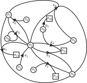
In order to allow the user to better understand how the utility–service provision problem may be described as a directed hypergraph, we will first consider a simplified scenario in which only a small number of utility products,services and devices are considered. The hypergraph created for this purpose is shown in Figure 1. The nodes, marked in Figure 1 with circles represent products: n1–Solar irradiation, n2–Electricity, n3–Food, n4–Rainwater, n5–Organic waste, n6–Greywater, n7 –Clean water, n8–Drinking water, n9–Seawater, while the rectangular nodes represent services: n10–Drinking water, n11–Clothes cleaning, n12–Full body cleaning, n13–Nutrition. In the adopted approach the product nodes are perceived as storages. The role of storage is to accumulate a given product under conditions where product supply or production exceeds demand and supply the product when demand exceeds the supply. Each edge represents a different device which transforms one or more products into other product or products, or into a service: e1–Silicon Photovoltaic system, e2–Electric hob, e3–Ultrasonic shower, e4–Shower with electric water heater, e5–Tap, e6–Rainwater harvesting system, e7–Washing machine, e8–Greywater recycler, e9–Ocean salinity power generation (reversed electro dialysis). Hence, our hypergraph representing a simplified utility–service provision problem consist of 9 edges and 13 nodes. This particular hypergraph is not acyclic which means that some devices use the same product as an input and output. In this case product n9 is used as an input and as an output by device e9.
A?directed?hypergraph?representing?a?simplified?utility-service?provision?problem
Problem formulation
Having such a utility-service provision solution space specified with the hypergraph in Figure 1 we can now search for possible candidate solution given the required services to be delivered and constraints put on products. In this example the required services are n10, n11, n12 and n13. The constraints are: product n2 cannot be delivered by the infrastructure and product n6 cannot be removed by the infrastructure. Natural products available locally are n1, n4 and n9.
Properties of hypergraphs used for defining transformation graphs
The next step after problem formulation is to find candidate solutions based on the topology of the utility– service provision hypergraph and with the requirements and constraints specified in problem formulation. Search for candidate solutions is directed towards finding an answer whether it is possible to deliver required services with available devices and under the given constraints. At this stage demands for services and maximum throughputs of the devices are not considered, only the topological properties of the hypergraph and the given constraints on the amounts of products to be produced and consumed.
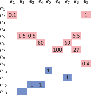
Definition of a transformation graph from the hypergraph is preceded by formulation of an incidence matrix which describes the topological structure of the hypergraph. For our simplified hypergraph shown in Figure 1 the color-coded incidence matrix is given in Figure 2. The storage’s product outputs, i.e., tail nodes are shown in green and have an associated value -1 representing a sink and thus input to the device. Storage product inputs, i.e., head node are shown in red and have a value of 1 denoting the source, i.e., output from the device. Grey-coded fields represent products that are used both as an input and as an output and have been assigned a value of 2. Finally, blue-colored fields denote the produced services and are have an assigned value of 1 as head nodes.
Incidence?matrix?for?the?hypergraph?introduced?in?Figure?1
The incidence matrix in Figure 2 shows that product n2 can only be produced by devices e1 and e9 (see row 2) and that product n6 can be recycled by device e8, as e8 is the input to n6. Therefore, these devices can be used to formulate the candidate solution, i.e., the transformation graph to comply with the constraints listed in the problem formulation section. Additionally, Figure 2 indicates that service n10 can be delivered only by device e5, service n11 can be delivered solely by device e7; service n12 can be delivered either by device e3 or e4 whilst service n13 can be provided by device e2.
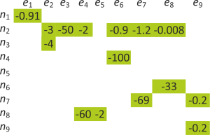
In addition to the incidence matrix, which provides information about the topology of the hypergraph, we introduce two more matrices which additionally provide quantitative information about the operating rules of the devices, i.e., how much of a product is used and produced by a given device. The benefit of such representations is that it enables a quantitative comparison of the amounts of products produced or used by corresponding devices and of the amounts of services they generated by the devices. This information can be later used to calculate the mass balances of all services and products and, subsequently, assess the feasibility of a given solution. Whilst Figure 3 presents the amounts of products (inputs) used by all devices Figure 4 shows the amounts of products and services produced by these devices. Since services cannot be used by devices as inputs they not included in Figure 3.
Inputs?for?devices?used?in?the?example?presented?in?Figure?1
Outputs?for?devices?used?in?the?example?presented?in?Figure?1
Additional information about a hypergraph, for construction of transformation graphs, is provided by a matrix of shortest paths from product nodes to service nodes, such as one listed in Table 2. Shortest path values in Table 2 are calculated with Equation 5. The matrix of shortest paths is used for solution optimization, e.g., when it is required to minimize the number of used devices. If the sought solution is such in which the number of used devices are reduced to minimum the devices chosen from the hypergraph to form the transformation graph should lie on the shortest paths. Another piece of information provided in Table 2 indicates whether there is a possibility to deliver a service starting from a given product node, e.g., when investigating the first column it is clear that there is only one path between the product node n8 and the service node n10. Also, by looking at the third row we can see that only the product n3 is required to satisfy the service n13. This could be an indication that, from the point of increasing resilience, it might be beneficial to add other devices that could deliver this service. Table 2 can also be used to highlight critical nodes or edges, i.e., the nodes or edges which if removed will prevent the required services from being delivered. Table 2 also shows that there are no paths between the product n5 and any of the services. Thus, the product n5 is not used by any of the devices in this example as an input. Apart from shortest paths between product nodes and service nodes the matrix of shortest paths can be also used to investigate how one product can be converted into another. Accordingly to our problem formulation, only the product n6 needs to be converted into another product. As it can be seen in Figure 1 this particular product can only be converted by device e8 into the products n5 and n7. Whilst information contained in either one of the representations is sufficient to uniquely define a graph, the incidence matrix and the matrix of shortest paths offer different and complementary descriptions of a graph.
Table?2
Shortest paths lengths in the hypergraph introduced in Figure 1
| n10 | n11 | n12 | n13 | |
|---|---|---|---|---|
| n1 | - | 2 | 2 | 2 |
| n2 | - | 1 | 1 | 1 |
| n3 | - | - | - | 1 |
| n4 | - | 2 | 2 | 2 |
| n5 | - | - | - | - |
| n6 | - | 2 | 3 | 3 |
| n7 | - | 1 | 2 | 2 |
| n8 | 1 | 3 | 1 | 4 |
| n9 | - | 2 | 2 | 2 |
Another parameter that is useful when analyzing a hypergraph (and therefore potential candidate solutions) is the cardinality of hyperedges, which in our hypergraph are respectively: e1 = 2, e2 = 4, e3 = 3, e4 = 4, e5 = 2, e6 = 3, e7 = 4, e8 = 4, e9 = 4.This parameter shows how many inputs and outputs are associated with each device. Information about cardinality of hyperedges can be useful at the stage of choosing devices for the transformation graphs. The size of the hypergraph is calculated as a sum of all its hyperedge cardinalities. Since the size of or hypergarph is 30 and it contains 9 nodes, a device has on average 3.33 inputs and outputs
Transformation graph definition
A candidate solution, i.e., transformation graph is formulated based on the requirements listed in the problem formulation in the section titled "Problem formulation". In principle, this problem can have many solutions and these solutions can then be evaluated and compared against each other from the point of view of their complexity, resilience, energy demand, robustness, etc. The first step in generating transformation graphs is to create an empty transformation graph containing all required service nodes, i.e., n10, n11, n12, and n13. In the next step the hypergraph presented in Figure 1 is traversed to find appropriate devices required to deliver the services specified in the problem formulation task. If, at any point, more than one device that fulfills these requirements exists, a number of copies of the transformation graph, equal to the number of devices fulfilling the same requirements, are created. In this example we start with two initial version of the transformation graph as two devices that can deliver service n12 exist in the utility–service provision hypergraph. Once all devices are connected, storage nodes for each product within a solution are added to facilitate subsequent dynamic simulation under changing demand and supply patterns with dynamic models generated from the transformation graphs. All storages are checked against the problem formulation to see whether each product can be delivered or removed by the infrastructure. Based on the problem formulation, product n2 cannot be delivered by the infrastructure and product n6 cannot be removed by the infrastructure. Therefore, a device that can produce product n2 is required. Again, there are two devices that can produce this product. Therefore, additional two copies are created.
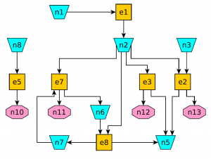
An example of a transformation graph is presented in Figure 5 where devices are given a rectangular shape, services have an octagonal shape and products are depicted with trapezoids.
Example?of?a?transformation?graph
Sensitivity analysis
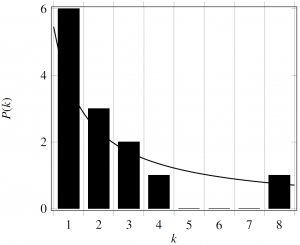
Sensitivity of a hypergraph to critical nodes can be described by degree distribution which provides the information on how many nodes in a hypergraph are highly and lowly connected. The more connections a node has the more important it is in the graph as more paths traverse through it. Therefore such a node may be critical to a proper functioning of a system described with such a graph. Figure 6 shows that the degree distribution for our hypergraph follows a power-law function P(k) ~ k-0.9335. As Figure 6 shows there are six nodes that have only one connection whilst one node representing electricity has eight connections. This indicates that electricity is crucial for the proper functioning of many, six to be precise (since two connections are electricity inputs not outputs), devices. Information included in the degree distribution of a hypergraph is very important in the analysis of the robustness of the solution as it helps in identifying the nodes that are critical for the operation of the solution system. Overall, the example presented in Figure 1 contains nine devices: two are producing electricity and six are requiring electricity to work, while one is independent, i.e., does not require electricity.
Degree?distribution?in?the?example?presented?in?Figure?1
Top betweenness nodes in our example are: electricity: , clean water:
, greywater:
. It shows that the highest number of shortest paths is traversing the electricity node since most of the devices presented in this example need electrical power to operate. However, since there are two devices, e1 and e9, that can produce electricity it is theoretically possible to deliver electricity to the system during a failure of a power grid. However, whether the amount of electricity provided from this second source is sufficient needs to be checked by calculating mass balances.
A complete utility–service provision model
The ‘mastergraph’, as defined in the Introduction, has the same structure like the simplified hypergraph presented in Figure 1 but with larger number of nodes and hyperedges. It is built from the database of devices obtained from literature and technical data sheets and is used to generate authentic transformation graphs (i.e., utility–service provision solutions) for real-life problems. At the current state of development the master graph contains V = 60 nodes (products and services) and E = 97 hyperedges (devices). This hypergraph can be described in the same way as the simplified example discussed in the previous section. However, due to high number of edges and nodes both the hypergraph and the incidence matrix would not be readable. Thus, we will omit the visual presentation of the hypergraph and its incidence matrix and instead we will discuss the other remaining parameters.
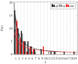
The size of our master graph is 299 with a device having, on average, 3.1 inputs and outputs. Degree distributions of the nodes in the master graph considering individually inputs (in), outputs (out), and total number of connected edges (all), are presented in Figure 7. The identified degree distribution for inputs as well as outputs follows a power-law function P(k) ~ k-1.109 (for node inputs: P(k) ~ k-0.9714 and outputs: P(k) ~ k-0.8215).
Analysis of the master graph led to the following observations. The most connected nodes are: electricity (total: 81, in: 28, out: 53), clean water (total: 19, in: 13, out: 6), drinking water (total: 16, in: 7, out: 9), greywater (total: 13, in: 11, out: 2) and waste water (total: 12, in: 3, out: 9).
Degree?distribution?in?the?mastergraph
Top betweenness nodes are: electricity: , clean water:
, greywater:
, drinking water:
. This centrality measure show which node has high influence on the transfer in the network, if the transferred item follows the shortest path.
Conclusion
This paper began with the examination of the relevant characteristics of the chosen utility infrastructures, i.e., real-world networks, such as water distribution systems, electricity grids, etc. These networks were reviewed using complex network analysis based on existing studies which investigated such properties of the networks as, i.e., topological features, robustness, redundancy, vulnerability (e.g., against intentional attacks), etc. The methods used in these studies were later applied to the analysis of hypergraphs describing utility–service provision scenarios.
Utility–service provision problem was formulated and presented with a hypergraph instead of simple graph as the hypergraph allows to map more than two nodes with one edge which is necessary to describe utility–service provision in which edges describe the devices which can use more then one product as an input and output. This hypergraph was then analysed with a number of statistical measures in order to extract additional information about the graph which is then used to generate candidate solutions, i.e., transformation graphs, which are subsequently used to specify dynamic models of utility–service provision systems which are then simulated and optimized - see 1,22 .
First the topology of the hypergraph is visualized with an incidence matrix which helps to identify the devices (edges) necessary to deliver the specified services (nodes) and the products (nodes) required for proper functioning of the devices (edges). This incidence matrix is then complemented with two additional matrices which, in addition to graph topology, also provide quantitative information about the amount of products consumed and produced and services produced in the system. Subsequently, yet another matrix, i.e., the matrix of shortest paths is produced to aid with identification of shortest paths between utility products and services, i.e., transformations requiring the least amount of devices. Additionally, the matrix of shortest paths is used to identify critical products required to deliver a specified service required for an assessment of the system’s resilience, i.e., its lack of vulnerability to situations where one or many products fails to be delivered. To assess the vulnerability of the system to failures of the devices we use both the matrix of shortest paths (which can be used to show the number of alternative paths to deliver the required service) as well as the cardinality of hyperedges which quantifies how many inputs and outputs, i.e., products and services are associated with this particular device. Finally, as the last measure of quantifying a hypergraph we calculate the node degree distribution which shows the critical nodes (with large number of connections) as well as its share in the total number of nodes in the system.
All of these measures offer crucial information for further analysis of utility–service provision such as generation of possible solutions (utility–service provision configurations), subsequent analysis of their resilience, vulnerability, robustness, and redundancy, and generation of dynamic models for the purpose of simulation and optimization.