Energy efficiency
In order to fulfill our obligations concerning CO2 emissions reduction, we need to reduce energy consumption and move towards renewable generation7, UKERC Energy Scenarios 205015,16,17,20,3. This will require a major transition in our society13,14,10,15,11. Much has been written on this issue21,22,6,4,18. Houses need an amount of energy and water to function7. The costs reflect the quantities required by consumers to attain their required levels of comfort, the profits and strategies of suppliers, and the wholesale costs of energy and water. The system we are considering therefore includes: people who live in various different types and sizes of house; the levels of efficiency in resource use of these houses; house improvement firms who will add insulation and improved appliances; utility companies; and potentially MUSCOs—Multi-Utility Service Companies19.
The importance of MUSCOs firms is how much they might be able to help us reduce our resource use and emissions of greenhouse gases. Instead of simply allowing households, house improvement firms and utility companies to interact alone, the emergence of a MUSCOs market would be to offer a service to households that both reduced demands on utilities and also supplied the energy and water required. The resource efficiency characteristic of a particular house can be the sum of that for each utility—Electricity, Gas, Water. The reduction in each adds up to the reduction for the house. The energy rating bands are A, B, C, D, E, F, G. So there are 7 grades officially (Energy Key, EPC, SAP). We have 10 in our model. 50% of houses today are in band D.
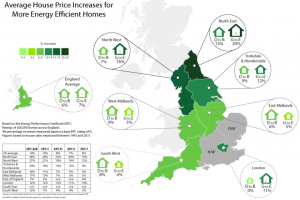
Average?house?price?increases?for?more?energy?efficient?homes
DECC Press Release 18/06/2013
The impact of a change from G to A or B is about 14% of the average house price for England, from G to C is 10%, G to D is 8%, G to E is 7% and G to F is 6%. But there are strong regional variations in house prices. For example, the North East improvement from G to A or B can lead to an increase in house price of 38%. This is partly related to the relatively similar costs of heating a house anywhere in the UK, but the widely different house prices in different regions. This gives us a way to estimate the ‘value’ of energy efficiency that is already perceived by people. For example, these changes in house prices are: North 38% and 27%; York & Hum 24%; East Midlands 16%; West Midlands 17%; East 7%; South West 12%; London 12%. For England as a whole it is 14%.
The average house price for England is 165k
North 127k
North West 121k
York & Hum 119k
Wales 134k
West Mid 147k
East Mid 135k
East 162k
South west 179k
South East 236k
London 275k
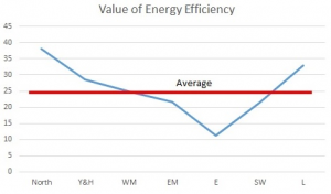
The?apparent?value?of?increased?energy?efficiency?for?different?regions
The average is around £25k
These figures give us a crude evaluation of how much strongly improved energy efficiency is already understood to be worth by the public. The figure would seem to be around £25k. This is of some significance in the calculations people may make in considering whether to pay for energy efficiency improvements or not. It is an additional positive reason to invest.
Houses start with a certain quality Q and cost and are attracted by suppliers that offer higher Q than cost. Q is related to the category h of the house. For example if 1 = very wasteful and only has a 10% reduction of use, h = 6 is good quality in that it uses 60% less resources. Later on we can map this on to the 7 energy efficiency ratings.
The key question is the cost of reducing the annual bill. Clearly, within each energy efficiency band there will be houses of quite different sizes that will have different sized annual energy bills, depending on their patterns of occupancy and particular demands. The attraction of increasing the levels of insulation and efficiency are therefore related to the percentage decrease in the annual utility bill that can be achieved for a given investment. The size of the investment required for a particular percentage reduction would be proportional to the size of the house.
As an example suppose the annual bill for a house is £1400. However, by moving the energy/utility efficiency from 20% to 60% the new annual bill would be £840 saving £560 each year. If the improvements cost £7000 then the annual savings, £560, are 8% of this investment. However the reduced costs will last for 30 or 40 years and so give rise to savings of around £20,000 in the long term. Clearly, if energy costs rise, as they will most probably, then the savings will be even greater. Not only that, the value of the property will also rise.
For some occupiers such as pensioners the bill will be high for the size of house and so the savings will more easily exceed the costs. For families with a low occupancy per hour then the savings may not be as great a proportion, and so interest rates will need to be lower for the cost of the action to be net positive. This could be modelled by allowing for a spread of behaviours and circumstances within each house type. We could have a probability for each type possibly reflecting different types of area. This could lead to a geographical version of the model that would be useful for the targeting of home improvement firms and of MUSCOs.
In general we can write an equation for the attraction of energy efficiency improvements for houses in each band of energy efficiency, even though they may differ considerably in size.
The overall attraction will be:
alpha(h)*Save% Annual Bill-Beta(h)*Cost*Int%
Cost is the cost of the ‘intervention’ which will be a function of the annual energy bill. The term Int% the interest rate for the loan of this cost. Alpha(h) will be a household parameter perhaps expressing their desire to save resources and Beta(h) will represent their desire not to pay too much. The more efficient a house is to start with the more costly it will be to make the same % reduction in consumption.
Each household improvement company will have offers available for households which can provide improved insulation, quality appliances and water saving techniques that will lead to a reduction in annual bills. If the house owner is able to pay for the improvements directly then the savings will be for them directly. If the house owner needs to borrow the capital for the initial investment then the amount of savings made will depend on the interest rate charged. The net adoption of these measures by customers will save them money but will also reduce resource consumption overall. There will be a population of households with widely varying consumption patterns. In addition there will be normal utility suppliers, direct ‘house improvement’ firms and also MUSCOs which will offer long term contracts as house improvers and suppliers of reduced quantities of utilities.
Initial model
In the situation under study we are starting from a low population of households with this action complete. But houses vary widely on their resource use efficiency and so there will be houses with a great deal to gain and others with much less. The model will deal with the changing level of household efficiency and resulting utility demands.
The initial distribution of houses might be:
H(0)=0, H(1) = 4, H(2)= 6, H(3)=8, H(4)= 5, H(5)=2, H(6)=1, H(7)=0, H(8)=0, H(9)=0, H(10)=0
Where the populations are in millions and come to 26million at present.
The household dynamics occurs as a result of customers choosing to invest in a house improvement scheme that will reduce resource use. The decision will reduce consumption at a given cost. The cost will be all the greater if the efficiency is already high as a result of previous improvements that have already been made. For example, increasing efficiency by 20% will be much easier and cheaper if the initial level is only 20% rather than 70%. Furthermore, if any intervention has a fixed cost then it will be more expensive to have 3 interventions of 10% to go from 30% to 60% efficiency instead of a single intervention from 30% to 60%. If we make a simple assumption that the ‘difficulty’ and cost of improving the efficiency increases with the level of efficiency already achieved, then each step of 10% more costs more and more. So, we choose a simple example of such a relationship, where if h represents insulation levels of 0, 10%, 20%……80%, 90% and 100% then the cost of moving 10% better goes up as 1/.9, 1/.8……1/.2, 1/.1, infinity.
At each moment a householder is in a house of efficiency h, and is looking at the costs of different possible further improvements. This tells us that the cost of improving a house from level 3 to level 7 (30% insulation to 70%) which will result in a 40% reduction in resource use, 15.29 -4.79 = 10.5 where there is a fixed cost of 1 for the action and a variable cost depending on the percentage reduction sought is 9.5. A 40% reduction in a house that is already at h = 4 is: 13.83 including a fixed cost of 1. In other words it gets more costly to improve houses the better they already are.
Table?1
The different costs incurred in improving the efficiency of houses resource use
The cost of an action to improve a house from 20% (h=2) up to 50% is a function of the size of the house and its particular occupancy, and this can be taken into account in an average way by using the annual bill as a measure of the costs involved:
Cost(h=2,Dh=3) = (10.46—3.36)*annual Bill = 7.1*annual bill
If we now consider that the reduced consumption is used to pay for the improvements then we see that the relative cost, the value for money, of each action is given by dividing the value in the table above by the size of the change in efficiency category. Each cell in the table (1) expresses the cost of reaching a particular level of efficiency of the house and the savings (0% to 100% of the annual bill) that this will represent. Because of this we can use table (1) as the basis for estimating the ‘attractivity’ of attaining each cell that results from the relative costs of the savings achieved. By dividing the cells of table (1) by the level of efficiency achieved, we therefore get table (2) which shows the pattern of attractivity that results from the balance of costs and savings, and therefore provides a transition probability for the household dynamics.
Table?2
The relative value of different improvements considering costs per % gain
The numbers in bold indicate where the best value for money would occur any house at a level i. For example, a house at level 2 (20% more efficient than nothing) the best value would be an offer to reduce the consumption by a further 20% to category 4. If we use the table 2 as a basis for the decisions that house owners make, then we can look at the probability of any particular step to the right (improved % efficiency) and downwards depending on how many separate interventions are used.
If we consider the rate at which improvements are commissioned to take a house from i% efficiency to j% then we see that houses in slice i% receive entrants from all less efficient values from:
0% to (i-1)% that is from H(0) up to H(i-1)
The numbers of houses in slice i% is diminished by the decisions to improve them and take them to all the possible ‘destinations’ of (i+1)% to 100%, and we can make the probability of each of these step according to the table 2.
The transition probability of going from i to a higher value j (from i+1 to 10):
T(i, j) = S * H(i) * Y * EXP(-r * cost(i , j))
Where S is the interaction between houses and firms and Y is the number of firms. These firms are more ‘house improvement firms’ than utility companies.
We can calculate the sum of all the probabilities from I, SumT(i), and use it to normalize the transition probabilities. Let us consider the change in the number of households of efficiency i% per year, DH(i). The households moving up from j to i are:
And for households leaving i for higher efficiency k are:
The +1 in the denominator avoids infinities. The firm/householder interaction rate that delivers improvements may be limited by the number of potential customers being vastly greater than the number of firms' agents able to carry out the work. If the time, Tau, taken for an improvement contract to be signed and carried out, then Tau is greater than S*H(j) and the rate of improvement is simply limited to the number of firms agents available. But if Tau is small then the rate of house improvement is affected by the rate at which new potential customers can be found.
Take i = 4: It has input from improvers from 0,1,2,3 and output from i = 4 towards efficiency levels of 5, 6, 7, 8, 9, and 10.
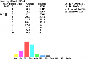
The initial condition for the simulation in figure(3) is based approximately on the UK in 2010.
The?initial?distribution?of?houses?among?the?resource?efficiency?0%?to?100%
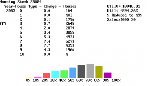
The model then can be run for successive intervals of 10 years as the houses are upgraded and gradually move up the categories of efficiency. After running the model for the equivalent of forty years, the distribution of households has changed considerably and we find the result of Figure (4).
After?40?years?the?distribution?has?a?resource?use?49%?of?the?initial?value
The model behaves reasonably and so can now be developed to allow for the growth of the home improvement industry as profits allow growth of the number of house improvement firms, Y, and in turn increases household energy efficiency.
We can now allow firms to have different strategies of profit and of quality of their actions, and see that this allows us to simulate the transformation that MUSCOs might offer. We could also allow for the different numbers and types of occupants as well as house types so that the detailed pattern of take-up can be simulated.
Modelling competition between utilities and MUSCOs
The idea now is to add MUSCOs into the model above. The dynamic model above concerns the actions of house improvement firms called in by households to reduce the utility bills. Obviously, households that make their own improvements are customers of ‘normal’ utility companies. So, the model above involves households, home improvement firms and normal utilities. Now we want to consider specifically as well as house improvement firms and normal utilities, the impact of MUSCOs which use long term contracts for utility supplies and also perform house improvements. This means that we shall have competition between ordinary Utilities and the Multi-Utility Service Providers. The main difference between the two is that while households can switch supplier fairly rapidly (3months?) if a household signs up to get house improvements and utilities from a particular MUSCO, then the arrangement will be at least 5 years, and possibly longer. This means that households, once they sign up are no longer ‘on the market’ for utility supply. Although getting a contract signed may take much more time for a salesman than simply getting a normal utility order, the fruits and the income are guaranteed to the MUSCO for 5 or 10 years. Their sales force efforts can be switched to non-contracted households. So, essentially both utilities and MUSCOs are trying to sell to the normal, non-contracted households. The advantage for a customer who signs up with a MUSCO is that there may be a discount on the house improvements offered and quite definitely the reduced cost of future supplies of energy and water.
In our model we shall simply use some trial (hopefully reasonable) figures to explore what happens. So in our equations the cost of moving from i to j is 80% for a MUSCO:
cost(i, j, 1) = Act(i, j) / j 'relative cost of i to j (j>i) Self Improvement
cost(i, j, 2) = .8 * Act(i, j) / j 'With MUSCOs cost of improvement is 80%
And the encounters that convert a normal household (H(i,1) into either an improved non-contracted one H(j,1) or into a contracted one H(i,2) are:
FOR i = 0 TO 10
SumT(i) = 0
'Rate at which H(i,1) is attracted to j (j>i) by offer 1 or 2
FOR j = i + 1 TO 10
T(i, j, 1) = S*H(i, 1)*Y1*EXP(-r * cost(i + 1, j, 1)) '
T(i, j, 2) = S*(H(i, 1) + H(i, 2))*Y2*EXP(-r * cost(i + 1, j, 2))
SumT(i) = SumT(i) + T(i, j, 1) + T(i, j, 2)
NEXT j
NEXT i
So, if we consider i = 4 we have Households in bands 0, 1, 2 and 3 that choose to upgrade to i = 4 and we have Households H(4,1) that choose to upgrade to 5, 6, 7, 8, 9 and 10 either as non-contracted H(j,1) households or as contracted H(j,2).
The?flows?into?and?out?of?band?i?=?4?as?households?upgrade?to?more?energy?efficient?bands
Although H(i,1) are converted to H(j,2) there is also a change in the other direction when the contract ends. So, H(j,2) households become H(j,1) after the contracted time. In other words they may retain the effects of house improvements (level j) but will lose the contracted utility supplies. They are then free to either buy utilities from ‘normal’ companies, or re-contract with a MUSCO. So, firms Y1 can only produce H(j,1) while firms Y2 convert H(j,1) into H(j,2). Therefore both salesmen 1 and 2 are only seeking H(i,1) and these must decline as H(i,2) increase.
Input to I 1 to 10:
Now we consider the net change in H(i,1) and H(i,2) as input minus households leaving i:
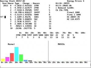
The resulting model gives us an evolution of household energy efficiency as shown in figures (6), (7) and (8). Here we have inserted an initial condition that corresponds with the data presented by DECC.
The?initial?condition?is?that?households?are?distributed?in?Energy?Efficiency?ratings?as?previously
As the model starts to run, there are improvements in the distribution of households both as simple buyers of utilities, who pay for their own house improvements and there are also customers captured by the MUSCOs who are signed up for long term contracts. They choose this solution partly because of the 80% discount they receive. However, since these contract do have to be renewed at some point, there is a slow ‘leakage’ from the contracted customers back to the non-contracted. The MUSCOs sales personnel must try to pick them up again.
After?20?years?there?are?nearly?equal?numbers?of?contracted?and?non-contracted?households.?But?Demand?has?fallen?to?42%?of?what?it?was?initially.
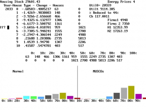
After?40?years?there?are?considerably?more?contracted?households?than?non-contracted.?Demand?has?been?reduced?to?30%?of?the?initial?level?as?it?is?the?higher?efficiency?levels?that?are?populated.
This model allows us to explore the effects of increasing or reducing discounts. In this model run it was assumed that it took 6 times as long for a salesman to get a contract signed than to simply arrange a normal switch of customer.
Conclusions
The model above seems to offer a good base from which to develop. The next stage will be to make the initial conditions those of the UK in 2014. We are also developing a ‘Multi-Agent’ version of the model in which customers and firms are agents and they can act individually in the model, allowing less use of ‘average behavior’. The further development of this systems model here will study the effect of having more than one MUSCo, exploring the effect of different strategies on their growth and success. In addition it will be necessary to model the mechanisms that generate profits for MUSCos, so that competing MUSCos will have to take into account not just what pleases customers, but also what brings in profits.
It would be good to know the progressive effects (% reduction in heat losses or in energy demand) of better (thicker) insulation, and improvements possible in appliances (Boilers, washing and dishwashing). In addition to these ideas instead of just modeling the ‘demand’ side of households we can also consider the competing companies that will offer different possible ‘bundles’ of services to households. The MUSCOs could use different strategies such as different contractual lengths, different discount rates and different profit margins. After that we can also model the market dynamics of competing companies with different types of offer for potential customers, varying from simple utilities selling units of resource to MUSCOs offering energy, water and ICT bundles as services provided under specific contracts. These can provide the kind of % reductions in demand seen above, and in addition will lead in the longer term to improved design and longevity of appliances. These different competing kinds of business offers can be modeled and the policies and actions and changing circumstances (subsidies, rising energy costs, etc.) can be explored and advice provided on the ways that the overall system can maintain comfort and convenience levels while greatly reducing carbon emissions, energy and water consumption. The transition towards a ‘leasing’ and ‘contracted service’ type of operation can be modeled as well as the long term consequences for design, maintenance and overall efficiencies. In many ways we shall need to consider the changing ‘life cycle analysis’ of the whole sector and try to see how carbon emissions and energy and resource efficiency can be improved in a sustainable way.