Introduction
Nonlinear dynamical systems theory (NDS) consists of a group of mathematical concepts for explaining and predicting how events change over time and the interrelationships among those concepts. The primary NDS phenomena are attractors, bifurcations, chaos, fractals, self-organization, catastrophes, and agent-based models. “Chaos” shows up in numerous political writings, denoting a state of disorganization, which is often in contrast to an old order of things that no longer exists. The objective of this article is to explain some of the formalities of mathematical chaos and some applications where relationship of chaos to conflict situations have been studied, and to isolate prototypic patterns of chaotic events that are inherent in some conflict situations.
Before continuing it is fair to point out that there are other NDS constructs that are useful in explaining some types of conflict situations. For instance agent-based models illustrate how individuals working in their own self-interest produce self-organized systems as they interact with other individuals. Self-organized systems often manifest sudden and discontinuous changes that are recognized as catastrophes or phase shifts (Guastello, 2002). Competition-cooperation dynamics are often inherent in those dynamics (Axelrod, 1984; Maynard-Smith, 1982).
Chaos
Chaos is a phenomenon that we can observe in a time series of events where seemingly random events are predictable with simple but special equations. The phenomenon was first discovered by Henri Poincare, a physicist, who was trying to solve the three-body problem in the 1890s: If we have a speck of dust moving between two gravitational forces, what is the particle’s path of movement? He concluded that the path would be very complex, such that the mathematics needed to describe it did not exist at the time.
Chaos regained notoriety in the early 1960s, when Edward Lorenz (1963), a meteorologist was studying weather patterns using variations of equations for turbulent flows of air or water. He discovered that very small differences in initial states of the weather system could produce some very different results and patterns. This is the principle of sensitivity to initial conditions, which became known soon afterwards as the butterfly effect (Smith, 2007; Sprott, 2003). A substantial amount of mathematical research on chaos was performed soon afterwards, and seemed to reach its peak in the 1980s. Most of the fundamental applications of chaos for explaining events in the social sciences started in the early 1990s.
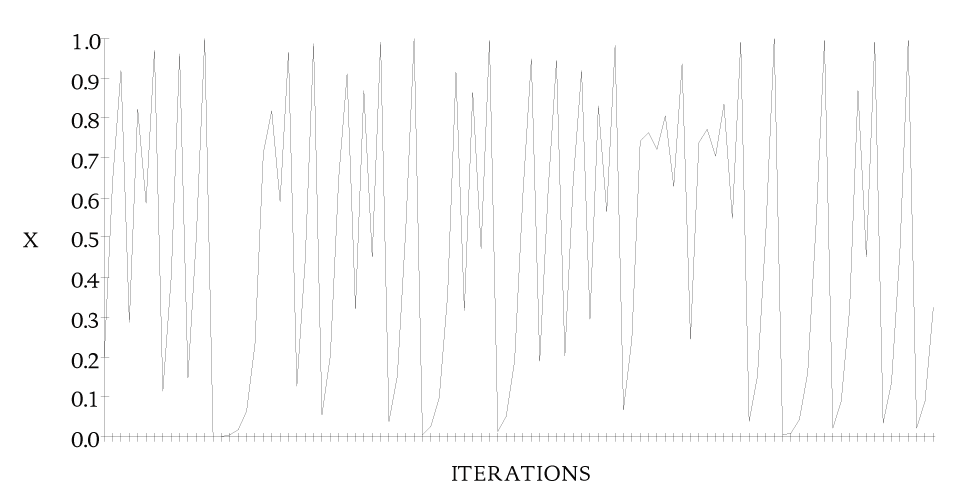
Chaos has three distinctive features. The first is non-repeating sequences; an example appears in Figure 1. The second is boundedness; the values of the variable being observed stays within a fixed range, even though the movement within the range is unpredictable. The first two properties are really matters of degree.
The third feature is sensitivity to initial conditions: Two points start arbitrarily close together, but become far apart as iteration progresses. Iteration is a computational technique of starting with a number, running it through an equation, taking the result and running it through the same equation again, running the next result through the equation, and so on. It is convenient to regard the behavior of living systems over time as computations, even if the organism is not consciously doing any math.
Pathways to Chaos and Conflict
There are three basic pathways by which a system can become chaotic. The first is an application of the three-body problem. Figure 2 shows a more complicated example (from Borges & Guastello, 1996; Guastello, 2002) of an attractor field with three attractors (A1, A2, A3) of different strengths. The points labeled S are saddles, or compromise points between each pair of competing attractors. The opportunity for conflict here is that, if a point enters the field, it is pulled in different directions in an unpredictable way, as denoted by the tangled thread. A partial solution to the conflict between two attractors, which represent two arguable positions on an issue, would define saddles that could attract points from two directions. What
actually happened in the simulation is that a point that indicates the position of the solution entered the field in the neighborhood of A1, visited two of the compromise positions, and landed on A2. The implication, nonetheless, is that bilateral agreements are not going to resolve any conflict if there are three or more interest groups involved; A3 received virtually no attention even though it was as strong as A2. The odds of people changing their preferences for possible solutions often increases as the number of options and the number of interest groups increases. In fact, chaos is more or less guaranteed if there are four participants and four options (Rand, 1978).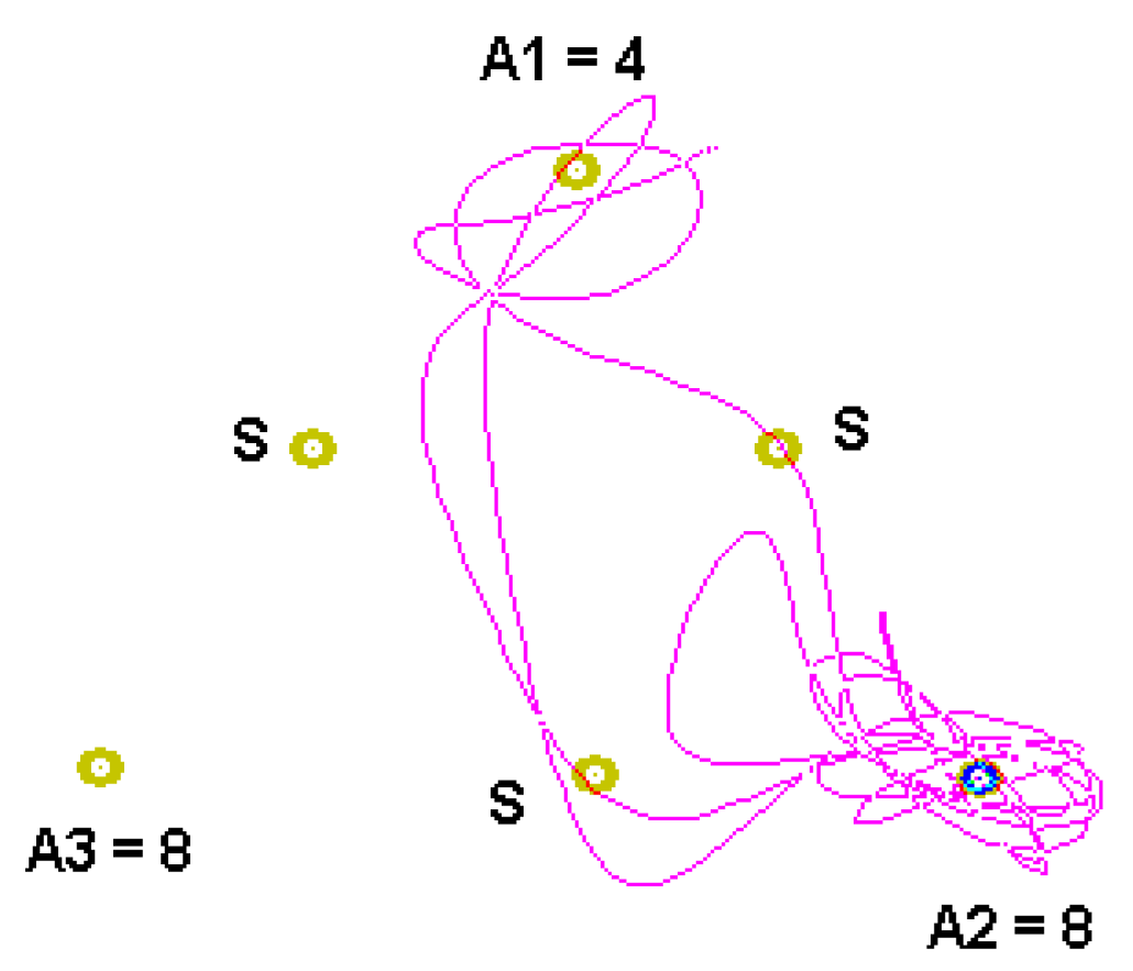
The second pathway involves coupled oscillators. A set of three pendula is shown in Figure 3. When Pendulum 1 oscillates, the middle one moves faster and its motion pattern becomes more complex than strictly periodic, and the third swings chaotically. The opportunity for conflict can be found in a coupled system involving, for instance, three organizations in a supply chain. Pendulum #3 does not like being jerked around, and probably cannot function well with all the entropy or unpredictability associated with the motion of the system it is experiencing. In human terms, the uncertainty associated with entropy is equivalent to the experience of risk, which the people or groups that reside later in the chain would like to control.
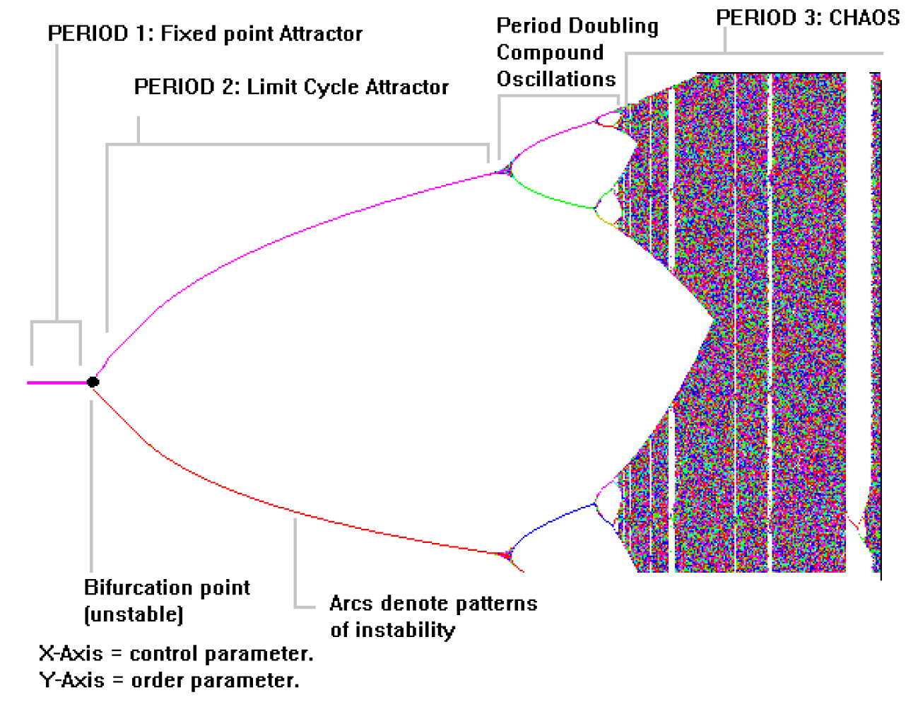
The third pathway to chaos (Figure 4) involves a bifurcation mechanism and a control parameter that increases the level of entropy in the system. When the value of a control parameter passes a critical value, the system oscillates instead of remaining stable. As the value increases further, the oscillations become more complex, and eventually the system goes into chaos. The bifurcation model was a popular
Figure?4
The logistic map showing stable, oscillating, period-doubling, and chaotic regimes as the value of a control parameter changes.
On the one hand, the bifurcation mechanism explains how to unravel an otherwise stable system in order to make some needed changes. It also characterizes a group exploring ideas for change that could be opposites of each other. Eventually one would need to reverse the control parameter to bring the system back to stability. On the other hand, the self-organizing process should return the system to relative stability automatically.
Finding Patterns with Symbolic Dynamics
There are actually a few dozen known mathematical systems, all with different equation structures, that produce chaos (Sprott, 2003). It would be virtually impossible to frame a research problem a few dozen different ways as required by each one of the models to see if anything resembling chaos was apparent in the data. Typically problems are defined and understood at a more elementary level, which leads to the same concern. An overview of two types of data analysis strategies that can be used to find patterns in data follows next. The first involves the use of symbolic dynamics and a specific technique called orbital decomposition (Guastello et al., 1998; Guastello, 2000).
Symbolic dynamics is a mathematical area devoted to finding patterns in qualitatively defined events. Orbital decomposition is one of those techniques. It is based on the idea that a time series of events could be as complex as chaos and that the chaos can be decomposed into periodic functions, which are the orbits, that are all intertwined with each other. The procedure begins with a series of qualitative events that can be coded into categories; the system of categories is dictated by the research topic. Each event is given a letter code. The algorithm finds the optimal length of a series of events, entropy statistics associated with it. The metrics include a Lyapunov exponent, which is a measure of turbulence, and fractal dimension, which is a measure of complexity, a ?2 test to determine whether the string patterns occurred by chance, a ?2 that describes the degree of fit between the patterns and original data, and the patterns themselves. It is also possible to code for two or more sets of categories simultaneously.
Spohn (2008) used orbital decomposition to isolate patterns of behavior that would explain the build-up of violence in four historically critical places: Yugoslavia after the break-up, South Africa during apartheid, Peru’s struggle with the Shining Path, and the ethnic confrontations in Gujarat, India. Each country’s events were analyzed separately; one goal was to compare the types of patterns that would emerge. Each event was coded for five different variables: the type of originator of the violent event, the action taken (acts violently upon, resists, etc.), the object of the violent action, the subject’s stage of violentization, and the object’s stage of violentization. Each variable consisted of several categories.
The results showed that there were indeed recurring events. The pattern lengths varied by situation. Yugoslavia’s were short, consisting of two events in a repeating unit. Peru and South Africa showed three-event sequences, and Gujarat showed four-event sequences. Fractal dimensions ranged from 1.2 to 1.7; higher dimensional complexity is associated with a greater variety of repeating patterns found. The following is one example of the seven 2-event patterns found in Yugoslavia:
Ethnic group retaliates violently against another ethnic group, both in full virulency, followed by UN/NATO forcibly halts violence by ethnic group; UN/NATO not involved in violentization process, combatants in full virulency (p. 105).
The following is one example of the twelve 3-event patterns found in Peru:
Government commits violent act on village or small association; government in virulency, community in violent subjugation or personal horrification, followed by two more instances of the same (p. 107).
The pattern indicates that the same event occurs three times before a different pattern would occur. A different pattern would contain a different combination of three events that recurs. A different event would involve a different perpetrator, different target, or different level of violent expression.
The following is one example of nine 4-event patterns found in Gujarat:
Community commits violent act on other community; instigator in virulency, victim in beligerency, followed by three more instances of the same (p. 113).
Pincus (2009) also used the technique in several studies to assess conflicts within families or other groups. His research strategy was to record conversations, code each utterance for one or more variables of interest, and then apply the orbital decomposition calculations. The patterns that resulted from the analysis once again had a great deal of diagnostic value.
Structural Nonlinear Regression Equations
Next, let us consider the case where we have some continuous variables, but once again need some sort of a generic approach to analyzing the possible dynamics instead of a gunshot analysis of a few dozen possibilities for chaos alone. For this purpose we can rely on a small number of possible equations that we can test through nonlinear regression using standard statistical software packages, such as SPSS (Guastello, 1995, 2002, 2005). There are four basic models in the set, and they are all functions of e.
We can consider the first two here. Equation 1 is a simple exponential function. Equation 2 contains an unknown bifurcation variable. The procedure would be to test both models, compare R2 for Equation 1, Equation 2, and also usually for a linear model, or any other competing theoretical model that happens to be pertinent. In Equation 1,
z2 = exp(?1z1) + ?2 (1)
?1 is a nonlinear regression weight. ?1 is the statistical equivalent of the Lyapunov exponent, which indicates the level of complexity and turbulence. If ?1< 0, the time series is veering toward a fixed point attractor. If ?1> 0, chaos is present. The fractal dimension, Df = exp(?). Note, however, that even though an analysis with Equation 1 can ascertain the presence of chaos, Equation 1 (with the estimated parameters) is not chaotic itself if it were to be iterated over time. Nonetheless, if we know z1, it tells us what z2 is going to be even under chaotic conditions, assuming that the model actually fits the data. Johnson and Dooley (1996) showed that Equation 1 provides very reasonable estimates of the fractal dimensions associated with data generated by the Lorenz and Rossler systems, which are well-known chaotic attractors.
The second model in the exponential series contains an unknown bifurcation effect, which indicates the presence of a variable that affects the inflection of the curve:
z2 = ?1z1 exp (?2z1) + ?3 (2)
If ?1 is sufficiently large, we can observe oscillations, period doubling, and chaos if we were to iterate the function over time. It is essentially the May and Oster (1976) model for population dynamics, which is a transformation of the equation for the logistic map shown in Figure 4.
The structural equations technique with nonlinear regression has been used in numerous studies. An application to a conflict situation is considered next, involving international political polarization and the magnitude of war (Guastello, 1995). The measurements of polarization and magnitude of war for the years 1865-1974 were taken from data published in Moul (1993). As a benchmark, the cold war years were often polarity values of 2, representing the US and USSR, and 3 when P. R. China was a political actor. Historically polarization was commonly interpreted as a predictor of war in the short-term. Its opposite is multipolarization.
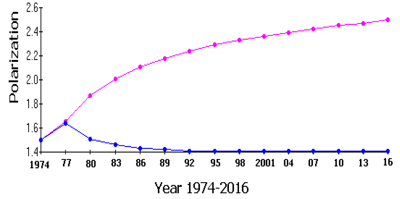
The results for the analysis of polarization showed the Equations 1 and 2 were equivalent in accuracy (R2 = .62). The next step was to iterate the functions into the future to see if they would produce similar forecasts. The Lyapunov exponent was positive in both equations. The results of that analysis appear in Fig. 5, and the two functions predicted some very different futures. Equation 1 predicted a sharp, then gradually increasing upward trend toward multipolarization. Equation 2 predicted an upward blip, followed by a drop in polarization levels, roughly equivalent to the cold war scenario. The actual events of the early 1980s did indicate that two futures would be possible, depending on whether the US adopted the Space-Based Defense system (a.k.a. the “Star Wars” plan), which would have been enormously expensive for either the US or USSR assuming that it would actually work properly. President Reagan pushed the plan on behalf of the US, and the USSR dropped out of the competition due to lack of funds and its own internal political concerns. The rest, as they say, is history, and the course of world events tended toward the upper curve.
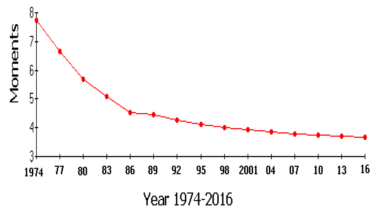
The results for the magnitude of wars between countries showed that Equation 2 was the better model (R2 = .41). The Lyapunov exponent was negative, signifying a trend toward asymptotic stability (Figure 6). The forecast showed a steady decline in magnitude, which appears historically accurate today. The data set did not reflect internal civil wars or terrorist events, however. I will return to polarization dynamics a bit later.
Arms Race Dynamics
Sometimes two agents pursue their own interests and find themselves in serious conflict that escalates. They are probably competing with each other over something. The cold war and arms race of the 1950s-1980s is a dramatic case of an escalating potential for conflict. Richardson (1960) developed a mathematical model for the situation, which Mayer-Kress (1992) analyzed further, noting that the Richardson model was an extension of the logistic map:
xt+1 = xt—k11(xt—x0) + k12(1-xt) (3)
Figure?5
Forecasts of international polarization. Reprinted from Guastello (1995: 383) by permission from Taylor and Francis.
Figure?6
Forecasts of magnitude of international wars. Reprinted from Guastello (1995: 384), by permission from Taylor and Francis.
yt+1 = yt—k22(xt—x0) + k21(1-xt) (4)
where x and y are the expenditures of the two countries, k11 and k22 are forces that control their expenditures to pre-race levels, and k12 and k21 represent the speed of the growth in hostilities. Mayer-Kress found that the expenditures remained stable if k12 and k21 remained below a hypothetical value of 3.0. If either parameter exceeded 3.0, however, the system went into chaos immediately, and did not stop at the intermediary dynamics of oscillation or period doubling. It was also possible to extend the model to three-nation systems, or to systems involving three types of armaments—offensive, defensive, and anti-defensive.
Polarization in Groups
The notion of polarization at the international level leads to the question of what dynamics could be involved in polarization within relatively small human groups. Polarization is often connected to conflict in groups, either as a starting point, or as a high-water mark of the group’s activities. The process of polarization itself is not chaotic, however; other dynamics are involved.
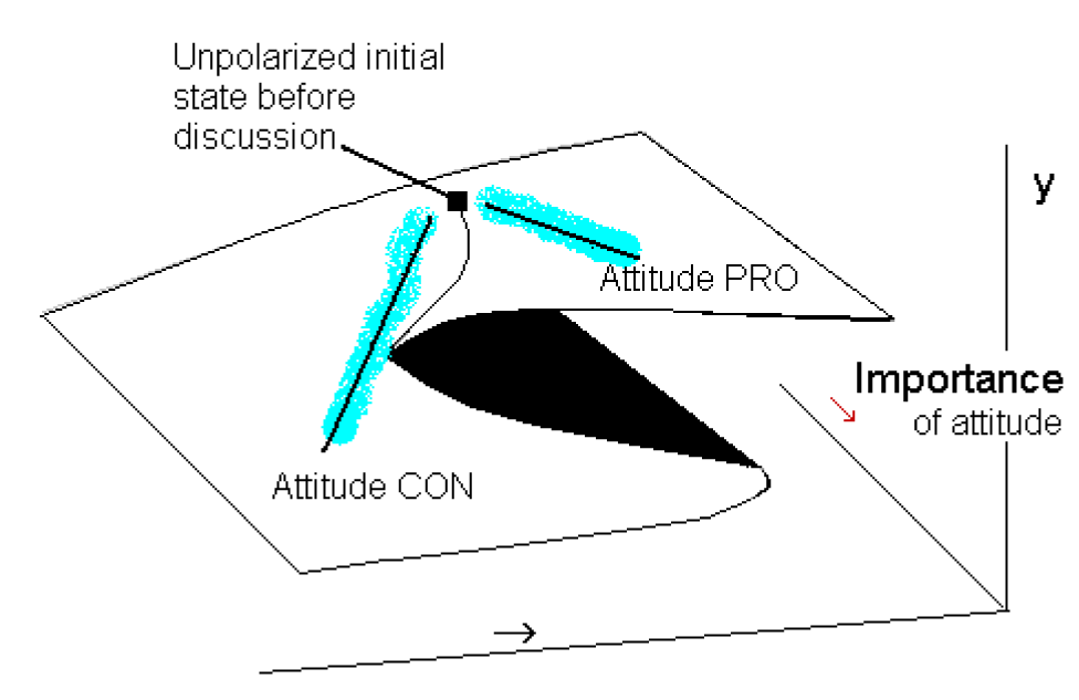
Groups often discuss their ideas, plans, and attitudes and find they have differences of opinion. In cases where the participants are not too emotionally involved at a personal level, they often find midpoints or compromise positions that are agreeable to most participants. If the topic or attitude target is “important,” however, continued discussion will lead to polarization of group members, rather than compromise. Latane (1996) expressed the dynamics as a cusp catastrophe model (Figure 7). The cusp catastrophe model is one of seven models that intrinsic parts of a comprehensive theory of discontinuous events (Thom, 1975; Zeeman, 1977). The response surface shown in Figure 7 shows the range of places that a system may occupy along a behavioral variable, y. The response surface contains some distinctive pleats or cliffs, however, and movement across those cliffs produces dramatic qualitative change. The shaded region represents the range of locations where the system is very unlikely to go. The shaded region is a repellor: points move away from it, instead of toward it as with an attractor. There are two stable states (attractors). The group begins at the unstable point (a saddle) on the surface and then splits into distinctive poles if the importance of the attitude is high, and does not polarize for less important attitudes.
Given that an attitude is important, the cusp model also indicates, as part of its intrinsic dynamics, that some people could waffle between the two poles before locking in to one attractor or another. The waffling process is more formally known as hysteresis, which is depicted in a two-dimensional display in Figure 8.
The cusp model also contains a second control variable (asymmetry) that corresponds to the horizontal arrow in Figure 7, which would govern whether a person would shift attitude toward one pole or another, or decide to join one coalition or the other. A candidate for the missing variable was later identified by van der Maas, Kolstein, and van der Plight (2003) who separated a construct of political orientation from attitudes toward a specific group of
policies. They were able to fit the political orientation variable to the asymmetry control parameter, with the attitude toward specific policies used as the behavioral response. Arguably those two constructs might be similar enough to be considered redundant. The cogency of the arguments from the group favoring one pole or the other could be influential on undecided people in much the same way as the perception of an ambiguous figure is influenced by the quantity and direction of specific details in the drawing (Stewart & Peregoy, 1983) or a jury’s decision could be influenced by the quantity, cogency, and direction of specific details in a litigation (Guastello, 1995).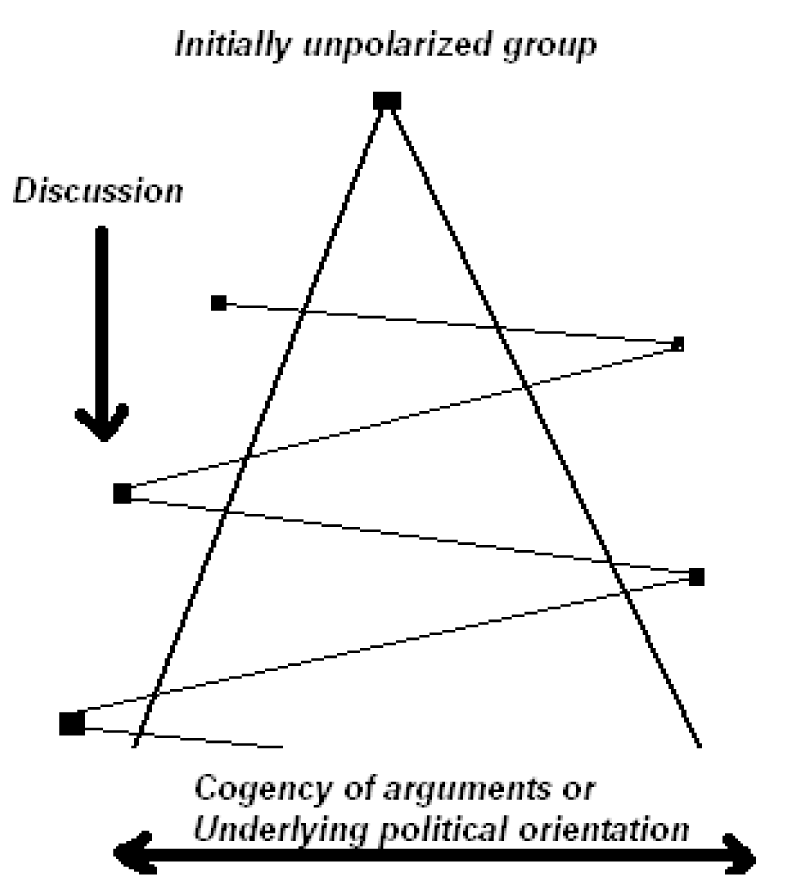
The important point for pattern recognition is that hysteresis is an unstable pattern, but it is not chaos, and not the same as the three-body problem. For one reason, the two attractor bodies in group polarization are in the process of forming during the discussion. The second reason is that there are two control parameters governing the shift between the two attractor bodies. One control parameter determines the size of the shift at a given moment. The other influences direction; neither type of control parameter exists in a strict three-body problem.
There is also a third reason, which is that there is a repellor force in the cusp model that is located in the dark shaded area. This is a place where very few points are likely to fall. It naturally moves agents away from the shaded location to somewhere else, which happens to be the attractor structures.
Summary
Several patterns of conflict have been identified here that involve chaos. (1) Multiple attractors produce conflicts of approach, typified by a light-weight object trying to maneuver between two gravitational forces. (2) In a series of coupled oscillators, the oscillator at the end of the chain experiences the greatest uncertainty, which is often characterized as risk in human terms. (3) There is an underlying order in chaos, and it is possible to identify patterns of events in high entropy situations using symbolic dynamics techniques such as orbital decomposition. (4) Similarly, it is possible to harness a prediction model for continuously-valued events and forecast future trends. As with all forecasting systems, there is an assumption that the underlying order of things is not changing. (5) Escalating hostilities or competition can be characterized as variations of the logistic map pathway to chaos. (6) We considered a negative example of chaos that involved polarization in groups. The instabilities underlying the polarization process are aptly described by a cusp catastrophe and are not chaotic, unlike the polarization of nations over time.