Introduction
In the hereby presented article, an agent-based model of population dynamics for the European regions at NUTS 3 level is discussed. Before proceeding to the presentation of the model details and description of the preparation of the data bases needed to feed and calibrate this model, let the latest advances on this topic be presented. Thus, we will introduce how agent-based models have been used to model the population dynamics, paying also attention to the importance of labour market.
Nowadays, population dynamics is the field of study of the highest interest. It joins the results extracted from the economics, demography studies and sociology. All of them have their own methodologies of studies and all of them present new techniques of population dynamics and related phenomena modelling1,2.
In “Semi-Artificial Models of Populations: Connecting Demography with Agent-Based-Modelling”3 the authors present a seminal paper of an agent-based model of the dynamics of mortality, fertility, and partnership formation. They “propose that directly linking demographic methods with ABM frameworks will allow us to produce models which increase our understanding of population change, while simultaneously helping us to avoid the pitfalls of an over-dependence on empirical data. ABMs allow us to produce models which have a greater explanatory capacity, while the demographic components allow to use the inherent flexibility of the ABM approach to generate plausible scenarios within a given parameter space”. In this article they present an agent-based model that emphasize on the partner formation and they combine it with survivorship and birth rates empirical and projected. Our agent-based model, developed at the same time, follows the same path and develops an agent-based model with the same features as the cited one, but ours is focus on the importance of the labor market and migration patterns. These two relevant parts are not taken into account by Silverman and his co-authors, but they may be fundamental in economies as the ones of PIGS countries, where the long-term unemployment and the inexistent recovery expectations urge a part of the population to change their location. Hence, migration patterns within European countries also affect the overall population dynamics. These patterns have been incorporated in MULTIPOLES model. It has represented an important step in the next generation of models to study the population dynamics, and it includes births and deceases and migrations, improving the results obtained by the official statistics services4.
The key feature that has not been taken into account in the paper previously mentioned was the importance of migration. Nevertheless, the study of migration dynamics has been modeled according to the agent-based approach premises recently. The ABM technique is one of the most promising techniques that have been used in population and labor market modelling. In the report “Agent-based modeling of population dynamics in municipalities: Migration in the Derbyshire & Nottinghamshire cases in the UK”, written by Q.Zhang and W. Jager5, the model allows the agents making a decision whether to migrate or not. This approach undertaken in the PRIMA project (EU 7th FP) follows partially the same track undertaken by MOSIPS project6, and hereby presented in this parallel developed model. The scope of PRIMA and this model are widely divergent, and this difference has a counterpart in the variables and methods used in both of them. The aim of PRIMA model is to study the migration dynamics in 14 wards (low-level election unit) in the UK while the model we are presenting covers the European regions at regional level and its aim is not only to model migration but the interrelations between labor market interactions, migration decisions, education demand and demographic processes in order to achieve a correct scheme of how these different decisions are interrelated and they affect the population dynamics.
One of the most important techniques that has been used in study of population dynamics and especially labor market policies incidence are the micro simulation technique and agent-based modelling. As Rahman et al. underline in their paper “Simulating the characteristics of populations at the small are level: New validation techniques for a spatial micro simulation model in Australia”7, “these days spatial micro simulation modeling plays a vital role in policy analysis for small areas. Most developed countries are utilizing these tools in more effective ways to make acknowledgeable decisions on major policy issues at local level”. The authors apply this technique to study the housing stress phenomena and demonstrate its variability in accordance to changes in the geographical units under study. The main characteristic of this paper are not only the results extracted from the analysis, but the whole technique of micro simulation as well as a proposed validation technique to perform the statistical test of the SMM estimates based on Z-statistics and corresponding p-value. The concept of housing stress pointed by the authors has plenty of definitions in the literature, the most common is to consider it happens to a household that spend more than 30 percent of its income in housing. This concept makes us to highlight again the importance of the high unemployment rates in many European regions in the recent years. This high unemployment has meant a dramatic decrease in family income for a significant number of households. Moreover, in a number of countries a major portion of these families have to face the payments of a mortgage and subsequently the housing stress is a relevant phenomenon in the most affected countries by the current downturn.
Although the pure demographic topics and the population dynamics in general seem to be the areas of research of the prime importance, the interaction between demography and the economy growth and development is not less relevant. C. Elgin and S. Turnen in their article from 2012 “Can sustained economic growth and declining population coexist?” arise the questions whether sustained economic growth and declining population could coexist and if there is a possibility to reverse the decline in fertility. In fact, this is the question that has been raised in the hereby presented paper. The main conclusion obtained by the Elgin and Turnen is that returns to human capital in production can help us to understand that contradiction. Whenever the degree of increasing returns to human capital falls, developed economies can take advantage of the so-called endogenous efficiency-augmenting mechanism. Generally speaking, this mechanism describes the possibility of switching to “human capital oriented technologies that support aging population”. Taking into account that possibility, the coexistence of sustained economic growth and a declining population is allowed in the long run. The main finding of this research is that “the degree of increasing returns to human capital has been falling over time throughout the world along with population rates”. Our agent-based model takes into account this recent empirical finding and it is built foster a simultaneous increase of human capital stock when the long-term unemployment rises, as found in the empirical data, while the regional population can decrease due to the dynamics of mortality, fertility and migration. Thus, the micro analysis allow including certain aspects of major importance in the analysis of population and the impact economy and agent’s organization have on its dynamics8.
One of the most valuable article related to the topic of artificial labor market creation is the one written by A. Chaturvedi, S. Mehta, D.Dolk, R. Ayer: “Agent-based simulation for computational experimentation: Developing an artificial labor market” (2004) The authors of this article emphasized the usefulness of agent-based simulations in many areas of research and their huge applicability, including the labor market and population dynamics. In the article the creation of an artificial market (ATM) as an agent-based simulation model was discussed and two phases of ATM development were indicated: modelling and simulation phases. In the modelling one, the representation and specification are defined, while in the simulation, the scenarios are built to allow computational experimentations. The example implemented by the authors was the one of the military recruit market. The goal of this paper has been to underline the benefits of the ATM development that are, without doubts: supporting market segmentation and facilitating an integrated decision support functionality. Moreover, the agent-based simulations can be used to develop a platform for building an ATM that is commonly used to test different labor market policies incidence. Hence, the final goal is to program micro-level agent behavior that would have macro-level effects and that would, through specific calibration, reflect the economic reality. Moreover, the use of the so-called parallel worlds, specific interfaces used to switch from the real data to the virtual world, is especially useful during the scenario development and then during the decision making process for each of those predefined scenarios. The add value of this research was to elaborate a new methodological approach for building a large scale, macro-level synthetic economy, which works from artificial simulation life cycle principles, as well as to develop an effective representation techniques for synthetic economies, which supports market segmentation. The methodology applied by the Chaturvedi, Mehta, Dolk and Ayer, supposed a step in right direction in the labor market and population dynamics studies.
Overview
The aim of the agent-based model hereby presented is to forecast and simulate the population dynamics of the European regions at NUTS 3 level. In addition it makes possible to forecast the education demand of individuals and the labor market outcomes.These results can be displayed for different kind of individuals depending on their age, gender, nationality, education level and labor status.
In order to make possible these tasks, it is necessary to build a specific database. We make use of the population census carried out in 2001. In the near future it will be possible to have access to the microdata from the population census of 2011. It will make possible to extend the time scope of the model and to have two initial points, allow comparing the preserved heterogeneity of individual modeled data after ten periods with the actual microdata one.
Overview?of?the?model?and?the?needed?data?bases
https://emergence.blob.core.windows.net/article-images/2015/11/cd42e375-4f91-502f-b243-a11afb69ce54.png
This database built from the population census is used to initialize the model. Then every agent passes sequentially through the five implemented modules:
Aging and deceases: Every agent computes a probability of death and there are determined the ones who decease. Widowed and orphans agents are taken into account. The rest of the population increases its age in one year.
Education: The individuals can start, end and continue different levels of studies depending on their age, gender and labor status.
Pairing: Adult agents of one gender decide if they want to divorce, get married and have children.
Labor market: Individuals have the choice of turning into inactive or starting looking for a job. The labor demand is aggregately computed for every region and the hiring and firing processes are carried out accordingly the defined labor suitability of the agents.
Migration: The agents compute their satisfaction with their labor status and there is computed the probability of housing stress. Depending on the result the individual decides whether he stays in the same region or changes his location. In the second case, the family also changes its location.
An iteration of the system represents a year. After these five modules have been carried out for all the individuals the regional outcomes are computed in order to carry out the visualization. Then a new simulation cycle starts. The model is stopped after twenty iterations, making possible to simulate the actual results from 2001 to 2012 and forecast the trends from 2013 to 2021. This end point is set in eight years because our model uses a pool of macroeconomic forecasts of international institutions. These forecasts have been incorrect several times in the recent past because of the drawbacks of the used methodology9. We have computed the sensitivity of a deviation of +/- one percent in the growth of the GDP in all the regions during the first eleven iterations. In the worst case it had an impact of 5.23% of the overall population in a period of eight years (R0321 for the period 2004-2012). Then we set eight years as the maximum forecast scope of our model to control the uncertainty derived from the use of macroeconomic forecast. Nevertheless, other variables of our model, especially the labor market results are more dependent of this forecast. The associated uncertainty necessarily has to be higher than the boundary of five percent. The authors are aware of the efforts to increase the predictions time scope, but researchers must be conscious of the uncertainty of their presented results. A paradigmatic example of the pointed issue is the project “Population Pyramids of the World from 1950 to 2100”10 that after three years since its second version release it appears to be mistaken in plenty of its first results for the year 2015.
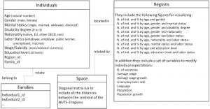
The model has following objects:
Individuals: These agents carry out the actions and populate the system.
Families: Individuals can be aggregated in families in a graph database. Families can decide together decisions such as migrate.
Regions: Individuals are located in one region and they can change their position. Regions include variables of aggregate outcomes and macroeconomic forecast.
Space: Matrix that includes the spatial distances between the centroid of every NUTS-3 region and cultural distances.
The INDIVIDUALS are the agents of the model. Their actual heterogeneity is preserved and included in the system in the following variables:
Class?diagram?of?the?agent-based?model
Age: The age expressed in years. It allows identifying dependent children: those individuals whose age is lower than the minimum legal working age. The age is the main variable that permits identifying different behavioral patterns in the system.
Curstud: It includes the education level in progress, otherwise is cero. When curstud is positive the individual cannot be part of the potential labor force.
Educlevel: It informs about the highest awarded diploma of every individual and it is used as a proxy of the human capital in the computation of labor suitability in the case of unemployed agents.
Gender: The Boolean variable adopts 0 for women and 1 for men.
Labstat: The labor status permits to identify if the individual is working or not (labstat=3 for employed agents) and whether he is looking a job (labstat=2 for unemployed) or not (labstat=1 for students and labstat=4 for inactive agents)
Labsuit: This variable is used to compute the labor suitability and hence reflect the probabilities of getting hired and fired in the iterations of the simulation.
Labperiods: The number of years since the last change in the variable labstat.
Marstat: It is another source of behavioral variation: 1 for single, 2 for married, 3 for widowed and 4 for divorced agents.
Nationality: The nationality is divided into native, other EU-28 and non EU-28 agents.
Satisf: The overall satisfaction of the individual current location. It is compared with the expected one in other locations.
Region_id: Region when the individual is located.
Family_id : Family identifier of the individual. It is not used in the hereby presented version of the model in order to simplify the presented model algorithms. This variable allows reducing the uncertainty in migration decisions, where all the individual of a household can change their location together when a family is defined as a couple and their children under the legal working age.
Every REGION has a set of variables that affects the behaviors of the individuals:
AVERAGE_INCOME: This variable is estimated using times series analysis and macroeconomic forecast information.
GDP_GROWTH: Actual data for the period 2001-2012 and macroeconomic forecast estimations for the remaining iterations.
Population: Total number of individuals in the database.
Popgrowth: Change in the population between the current and the previous iteration.
Urate: unemployment rate of the region.
Country: Country identifier.
The remaining objects are the FAMILY that includes identifiers of the individuals contained in them and the SPACE used to save spatial and cultural distances used to determine the migration patterns.
Initialization database
The model can be initialized in 2001 and 2011, corresponding to the times when the last two population censuses were carried out in the European countries. In addition to these databases, a set of additional data sources are needed to carry out the calibration of the agents behavioral rules, incorporated in the model with set of coefficients. The macroeconomic forecast it is computed with a collection of forecast changed as stated below in the section titled "Labor market".
National Population Censuses offer information of the population at municipal level for all the European countries, National Statistics Departments also supply microdata for a percentage of the population. The purpose of our model
Table?1
Variables obtained from the microdata of the Population Census
In addition to these variables this source has the household identifier. Our presented model does not require identifying families as groups of parents and dependent children (those who are under the legal working age) but the randomness level is reduced when this information is included. However, in the population census this information is not directly available. However, it is possible to identify couples and their children, and then arrive to the correct number and composition of families according to our definition. After correcting the errors and null values in the microdata, the rest of the population should be created in order to arrive to the actual population in every NUTS 3 region. Nevertheless, it would be incorrect to multiply each observation a number of times because it can be easily proved that, against the statement of the Statistics Offices, the microdata are representative of the population if we only take into account variables such as age and gender, but microdata do not represent the population when education level and labor status are considered.
Due to the previous mentioned reason, in the initialization process the agents are created and the values for the variables are defined according to this procedure:
Compute the number of individuals for each region in the year 2001 in the following groups: age (five years ranges), gender (male and female), marital status (single, married, widowed and divorced), nationality (native, rest of EU28 and others), labor status (unemployed, employee, inactive).
Each individual to be include in the database its subtracted to the aggregate value of his correspondent group.
The process ends when the results in each of the 1,440 groups of population.
It is not possible to compute the marginal groups in every case at NUTS-3 level. In these cases it is assumed a distribution equal to the one computed for the NUTS-2 or NCI’S-1 level.
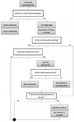
Activity?diagram?for?aging?&?deceases?and?education?modules
Aging and deceases
The aging and deceases module has two methods. In the first one every individual computes his decease probability and according to this probability he deceases or not in the subsequent one. Then, the individuals who continue in the population increase their age. This module takes into account the differences between genders, and how these differences vary with the age. It also includes the high morbidity probability that affects newborns.
In the second method when a person who had children passes away another individual in the same region and higher age become the new parent of the children. When a child is eliminated from the population his parents decrease in one their number of children.
AGING_1
Double deceaseprob
If age<1 and gender=0 Then deceaseprob= a1
Else If age<l and gender=1 Then deceaseprob= a2
Else If age<60 and gender=0 Then deceaseprob= a3 exp(a4age)
Else If age>=60 and gender=0 Then deceaseprob= a3 exp(a6age)
Else If age<30 and gender=1 Then deceaseprob= (a7 + a8 age) a3 exp(a4age)
Else If 30=<age<60 and gender=1 Then deceaseprob= a9 a3 exp(a4age)
Else If age>=60 and gender=1 Then deceaseprob= ( a10 + a11 age) a5 exp(a6 age)
End If
AGING _2
If deceaseprob<1000*mdm
If age<16
extract a number from N(a12, a13) = agemother
extract a number from N(a14, a15) = agefather
get a woman with age= agem,other and chidren>0 and woman.children - -
get a man with age= agefather and chidren>0 and father.children - -
Else If children>0
get an individual with same region, gender and higher age
set ind. children +=children of the deceased
Else if marstat=2
get an individual with same region, different gender and vnd.age-age=<|5|
set ind.marstat=3
End If
Individual -
Else
Age++ and Labperiods + +
End If
Education
The education module has two methods. In the first one if the individual is studying and he ends his studies he increases his education level and changes his labor status to unemployed. In the cases where he is studying and does not end the formation period, he just increases his counter of education periods and continues. Children of five years start the compulsory education.
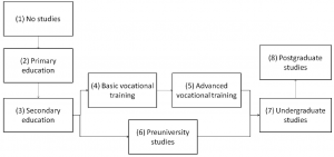
Education?levels?in?the?model
In the second method the agents who are not studying decide if they want to start the next level of studies or not. There are two possibilities: The usual path is to start the next level of studies just after ending the previous one. In addition, other people, mostly long-term unemployed, decide to increase their human capital to increase their chances to get an employment. Both circumstances are taken into account in this second method. In this way, a region with crises will increase its stock of human capital and it even could increase its GDP in the long run as stated in 11. The model assumes the education is a full-time occupation and it does not allow working and studying at the same time.
In the next figure it is shown how and individual can pass from the lower level of education to postgraduate studies. As it can be seen there are not backwards paths, as it is usual in the actual education trajectories. Once the individual ends the compulsory education (level 3: secondary education or high school) he can select vocational training or pre-university studies. Our model takes into account the different probabilities according to gender: Women start pre-university studies more often than men, who prefer to indicate vocational training.
EDUC1
If curstud>0 and (educ_level=l and periods_edu=24) / (educ_level=2 and periods_edu=40) / (educ_level=3 and curstud=4 and periods_edu=44) / (educ_level=3 and curstud=6 and periods_edu=48) / (educ_level=4 and periods_edu=48) / (educ_level=5 or 6 and periods_edu=60) / (educ_level=7 and periods _edu=80)
Then educ_level=curst,ud, Set curstud=0, labsta,t=2 and Labperiods=0
Else If curstud>0 Then periods_edu ++ Go to PAIRING_1
End If
EDUC_2
If educ_level=l and 5<age<16
Then curstud=2
If educ_level=2 and (age<16 | (unempl=1 and rndm<a16))
Then curstud=3 and labstat =1
Else if gender=1 and educ_level=3 and ((age<18 and labstat=3 and rndm<a17) | (unempl=1 and rndm< a18))
Then curstud=4 and labstat =1
Else if gender=1 and educ_level=3 and ((age<18 and labstat=3 and rndm<a19) | (unempl=1 and rndm< a20))
Then curstud=6 and labstat =1
Else if gender=0 and educ_level=3 and ((age<18 and labstat=3 and rndm<a21) | (unempl=1 and rndm< a22))
Then curstud=4 and labstat =1
Else if gender=0 and educ_level=3 and ((age<18 and labstat=3 and rndm<a23) | (unempl=1 and rndm< a24)
Then curstud=6 and labstat =1
Else if educ_level=4 and ((age<19 and labstat=3 and rndm< a25)
| (unempl=1 and rndm< a28))
Then curstud=5 and labstat =1
Else if educ_level=5 and ((age<20 and labstat=3 and rndm< a27)
| (unempl=1 and rndm< a28))
Then curstud=7 and labstat =1
Else if educ_level=6 and ((age<20 and labstat=3 and rndm< a29)
| (unempl=1 and rndm< a30))
Then curstud=7 and labstat =1
Else if educ_level=7 and age<27 and labstat=3 and rndm< a31
Then curstud=8 and labstat =1
End If
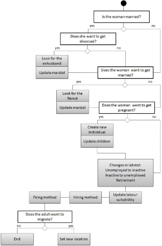
Pairing
Pairing In this module the individuals decide if they want to divorce, get married and have children. The model assumes a woman and a man form a couple. This assumption is made to simplify the model. Nevertheless, in next versions of our model this constraint will be removed in order to study- in depth the migration and reproductive behavior of same gender couples. In the paring module every married woman decide if she wants to divorce, then every non married woman decides if she wants to get married and if the choice is affirmative she determines the characteristics of her partner. Finally, every woman decides if she wants to have a new descendent. The specification of the module could be changed to include both gender decisions but the computations of the coefficients would be more complex and the results would not vary. In addition, non-married women take the decision of having children while the non-married men who have children are still infrequent.
Activity?diagram?for?pairing,?labor?market?and?migration?modules
The three activities undertaken in this module follow normal distributions according to the age of the ex-wife, fiancé or mother respectively. In order to compute the probability in each activity it is computed the area under the normal distribution in the range (age-1/2, age+1/2). The result of this defined integral is the probability of perform the indicated activity.
The nationality is taken into account through the different calibration of coefficients pointed as ?xx(nac) in the code. In this way the model takes into account the different probabilities of divorce, marriage and parenthood that every nationality has.
Finally, the model also takes into account the differences in the probabilities of getting married according to the previous marital status. At low ages, single, divorced and widowed have a similar behavior, but this similarities start slowly to diminish and divorced and widowed individuals tend to get marriage again with lower chances than single individuals. This fact takes place especially between women in countries of eastern and southern European countries.
PAIRING_1 //divorce
If gender=1
Go to LABOURA_1
Else If marstat=2 and rndm<?(age+0.5, age-0.5) N(a32, a33) a34(nac)
Then Marstat=4
Look for an individual with marstat=2, gender=1 and age-wife.age<|5|
Set marstat=4
PARING_ 2 //marriage
If (marstat=l and rndm<?(age+0.5, age-0.5) N(a35, a33) a37(nac)) /(marstat=1 and rndm<?(age+0.5, age-0.5) N(a33, a33) a40(nac)) / (marstat=1 and rndm<?(age+0.5, age-0.5) N(a41, a42) a43(nac))
Then Marstat=2
Look for an individual with marstat!=2, gender=1 and age-wife.age<|5|
Set marstat=2
PARING_ 3 //parenthood
If marstat!=2 and rndm<?(age+0.5, age-0.5) N(a44, a45) a46(nac)
Then Children + +
Create new individual
If marstat=2 and rndm<?(age+0.5, age-0.5) N(a47, a48) a49(nac)
Then Children + +
Create new individual
Look for an individual with marstat=2, gender=1 and age-mother.age<|5|
Set children + +
Labor market
The labor market is composed by two different parts: a real labor supply- integrated by individuals who decide whether to offer their workforce to the market or being inactive, and an artificial labor demand, computed adapting a set of standard macroeconomic rules.
Additionally to the hiring process, a number of workers are fired every period, becoming unemployed, this process is also determined aggregately through the expected macroeconomic outcome.
This module is composed by the following methods: labor supply update, labor suitability update and labor market.
In the first method every individual who is currently working decides if he is going to get retired. The main difference in this behavior comes from the gender difference. In most of the regions women tend to leave their jobs at a lower age than their male colleagues.
This different behavior is also considered when unemployed people cease to look for an employment. This behavior is especially remarkable when the woman is married and has children Unemployed individuals, independently of their characteristics, get inactive more often when the unemployment rate is high. In the same way, inactive individuals start looking for a job again in the expansionary phase of the business cycle the unemployment rate is low.
In the second method, after the updating of the labor demand, every unemployed individual update the value of the variable LABSUIT. It tries to faithfully represent the attractiveness of every individual for the labor demanders. A higher value increases the chances to be hired and decreases the probability of lose the current employment if the individual is employed. Nevertheless, in the third method, when the labor suppliers and the labor demand meet every individual has positive probabilities of been hired and fired, as it happens in the reality.
The variable labsuit has been calibrated with microdata of the Labor Force Surveys. It uses the values of the following variables of the individual:
Age: The labor suitability increases from the minimum legal working age to thirty/thirty five years approximately a twenty percent. It decreases at an higher rate and a worker becomes completely unable to find a job in the range sixty to sixty-five years old.
Gender: Males are hired with a higher probability. Male unemployment rate is lower and the labor suitability takes into consideration this empirical finding.
Nationality: Foreign workers usually have more difficulties to be hired.
Labor periods: Long-term unemployed population can hardly find a new job in most of the European labor markets, arriving to the so-called hysteresis. On the other hand long-term employees have less chances to be fired than the temporary workers, recently incorporated to the activity.
The variable labsuit is defined for employees and unemployed individuals, and it adopts cero value for students and inactive agents, making them unable to find a job. Its specification is different dependency of the labor status. For unemployed individuals it includes gender and nationality but these two variables are excluded in the case of current workers, who are assumed to not be discriminated for their personal characteristics.
Table?2
Labsuit parameterization for ES617 (Málaga)
| Coefficient | Estimated value (2001-2012) |
|---|---|
| ?67 | 63.842 |
| ?68 | -0.137 |
| ?69 | -0.086 |
| ?70 | -0.116 |
| ?71 | 0.028 |
| ?72 | 0.074 |
Table?3
Comparison of FC result with and without weighted past regional performance
If labstat=2 LABSUIT=Max (((a67age) - (age2)) (1+ a68foreigner) (1 + a69gender) (1+ a70labperiods) (1+ a71educlevel), 0)
If labstat=3 LABSUIT=Max (((a67age) - (age2)) (1+ a72labperiods), 0)
Else LABSUIT=0
These results show that in this NUTS3 region the unemployed foreigners have a 13.7% less chances to be hired than a native individual with the rest of the characteristics equivalent. Women have an 8.6% less chances to get employed than men. These effects can be compounded: A foreign woman would have a 23.4% less chances to be hired than a native man with the same age and periods unemployed. A higher education level, acting as a proxy of human capital stock, has also a positive impact on the chances of getting an employment. Finally, the last coefficient in each equation show that each year unemployed decreases the chances of getting a job in an 11.6% while each year being employed in the same company decreases the chances to lose the job in a 7.4%.
Finally, the labour demands at regional level are computed using a macroe-conomic forecast (FC) pool and adapting it to the past regional performance, overweighing the recent years.
In the example in the table 3, it is assessed the importance of weight the historic regional performance with respect to the national aggregate GDP increment (A). The two presented regions (A1 and A2) grew at a 92% of the national level. However, the first one increased its average while the second region results turned down. Hence, the weighted past performance (w(Ai/A)) makes use of this trend and predicts a grow forecast of the region 1 a 27.8% higher than the one of the Region 2.
With the regional forecast it is computed the change in the rate of unemployment according to the well-known Okun law, computed at regional level. This overall change in unemployment is divided into the regional figures for the number of employees to be fired and the number of unemployed individuals to be hired. The relation between these two quantities is considered fixed at regional level and is computed with the microdata of the Labor Force Survey.
Finally, in the artificial labor market mechanism, there are selected the workers to be hired and fired taking into account the relative value of their labor suitability and the number of vacancies and workers to be fired. It is assumed that the enterprises forced to fire their employees are the less productive ones, those that have a workforce with lowest values of labsuit. In addition, labsuit includes the number of periods the employee worked in the enterprise. Hence, recently hired workers are more likely to be fired. The workforce of new firms is included in this kind of employees and the model includes the well- known empirical finding of new enterprises have the lowest surveillance probability. Nevertheless, the matching process is randomized at individual level, but preserves the preference for individuals with a higher labsuit aggregately.
LABOR_1 //Labor supply update
Set Labstat=4 and Labperiods=0 If any of the following it is true If labstat=3 and gender=0 and age>55 and rndm<?(age+0.5, age-0.5) N(a50, a51)
Else if labstat=3 and gender=l and age>55 and rndm<?(age+0.5, age-0.5) N(a52, a53)
Else if labstat=2 and labperiods>2 and gender=0 and married!=2 and rnmd<?(age+0.5, age-0.5) N(a54, a55) ( a56 + a57urate)
Else if labstat=2 and labperiods>2 and gender=0 and married=2 and children=0 and rndm<? (age+0.5, age-0.5) N(a58, a59) ( a60 + a61urate)
Else if labstat=2 and labperiods>2 and gender=0 and married=2 and children >0 and rndm<?(age+0.5, age-0.5) N(a58, a59) ( a60 + a61urate) a62children
I flabstat=2 and labperiods>2 and gender=1 and rndm<? (age+0.5, age-0.5) N(a63, a64) x(a65+a66urate)
LABOR_2 // Update labor suitability
For every individual
If the nationality corresponds to the country that the region is included in Foreigner=0
Else Foreigner = 1
End If; End for
If labstat=2 LABSUIT=Max (((a67age) - (age2)) (1+ a68foreigner) (1 + a69gender) (1+ a70labperiods) (1+ a71educlevel), 0)
If labstat=3 LABSUIT=Max (((a67age) - (age2)) (1+ a72labperiods), 0)
Else LABSUIT=0
LABOR_3 // Labor market
Get hiredworkers=N
Order all individuals with labstat=2 decrea singly by labsuit
While Hiredworkers>0
If (N/number of unemployed)x(ind. labsuit/Max. labsuit)<rndm
Hiredworkers and Ind.labstat=3 and lnd.labperiods=0
Get firedworkers=N
Order all individuals with labstat=3 decrea singly by labsuit
While Firedworkers>0
If (N/number of employed)x(Min. labsuit/ind. labsuit) <rndm
Firedworkers and Ind.labstat=2 and lnd.labperiods=0
Migration
The migration module has four methods: in the first one adult individuals with housing stress decide whether if they want to migrate or not. In the second method every adult individual might decide to migrate in order to increase her income. Then they decide the destination region. The last method in our model takes account of the immigration phenomena.
Long-term unemployed individuals have the highest probability of emigrate, especially if they are young, single, they do not have children and they live in regions with a declining populations and high unemployment rates. Other kind of migration occurs in regions with low average income. In this case some individuals want to change their location in order to increase their expected income. Individuals who live in areas with declining population, an unstable work position, low age and no children are the agents who undertake this kind of migration more often.
Individuals who decide to migrate choose the destination location among the European NUTS3 regions. They computed the expected utility of being in every one of them, according to unemployment rate and population growth. Young individuals give more importance to the average income while elder ones prefer to migrate to a near region in spatial and cultural terms. This utility is multiplied by the population of the region to reach the probability of migration. The individual select a region randomly, but in line with this computed probability.
Finally, a number of immigrants (nonEU28 individuals) are computed for each region. This number depends on demographics indicators: population, immigrant population already settled and population growth, and economic performance: average income and unemployment rate.
MIGRATION_1
If labstat=2 and labperiods>2 and marstat=2
Search partner !=gender and |age-partner, age| <5
If partner.labstat=2 and partner=labperiods> 2 rndm<(a73 + a74urate)2 (a75 + a76popgrowth) (a77children)-1 (a78 +a79age)-1 Go to MIGRATION_3
Else Go to MIGRATION_2
End If
Else If labstat=2 and labperiods>2 and marstat!=2
If rndm<(a80 + a81urate)2(a82 + a83popgrowth) (a84 children)-1 (a85 + a86age)-1
Go to MIGRATION_3
Else Go to MIGRATION_2
End If
End If
MIGRATION_ 2
If labstat!=2 and rndm>(a87 + a88popgrowth) (a89 + a90age)-1 (a91 + a92labperiods)-1 (a93children)-1 Go to MIGRATION_3
MIGRATION_3
For each individual
For each region
Probreg=pop (a94 popgrowth) (a95 + a96urate)-1 + (a97 + a98age)-1 AVERAGE_INCOME + (a99 +a100age) (a101 cultural_dist) +(1-a102) spatial_ dist)
Order them, randomly
If probreg<rndm change location to this region
Else continue
End For; End For
MIGRATION_ 4
For each region
Nimmi= (a103pop+a104popnoEU28+ a105 popgrowth) ( a106 AVERAGE_INCOME +(1- a107)urate-1)
While Nimmi>0
Get an individual of the region with nationality=noEU28 and create a new record with the same characteristics except immi.agc=N(a108, a109)age
Nimmi -
If immi.marstat=2
Get an individual of the region with nationality=noEU28, gender!= immi.gender and create a new record with the same characteristics except immi.agc=N(a108, a109)age
Nimmi -
End If
End For
Calibration of the model
A set of data sources are used to calibrate every coefficient of the model:
The EU Labor force survey is a household sample survey that provides quarterly results on labor market variables of people aged 15 and over. In 2011 the quarterly labor force survey sample size across the EU was about 1.5 million individuals. This survey has available samples of microdata that make possible to compute plenty of the coefficients of the presented model at regional level.
Education statistics differ across the European countries, but every national Statistics Office includes the number of individuals studying and/or graduated in every education level. These figures are disaggregated at least by gender and age.
Migration statistics can be obtained through several ways. The most convenient ones to our needs are specific migration surveys focusing on the determinants and characteristics of the individuals who changed their location and municipal register that yearly computes the population classified by its characteristics (most of the times age range, gender, marital status and nationality).
Birth and decease statistics include information about the age and gender of the deceased and age. marital status and nationality of the newborn’s mother.
Wedding and divorces statistics collect information about the age of the partners. In several countries there are double entry tables combining the ages of the partners.
Calibration?of?the?coefficients?of?aging?and?deceases?for?PT171?(Grande?Lisboa)
https://emergence.blob.core.windows.net/article-images/2015/11/a6cbcd97-840b-ef44-3d75-3a73fb21b72f.png
In order to show how the calibration process takes place we use the case of the coefficients estimated with the decease statistics for the region of Grande Lisboa, Portugal (PT171). We start depicting the relation of the male mortality rate into female mortality rate (Fig. 6). We observe the usual behavior that follows three patterns (Figure 6, middle). Up to thirty years the mortality rate of the males increases with respect to the one for female individuals. From thirty to approximately sixty years its remains steady and since that age it starts declining. Three linear estimations were carried out:
ratio = 0.1171 age + 0.4727 (R2 = 0.7614)
ratio = 2.311 (series average)
ratio = -0.0492 age + 5.7332 (R2 = 0.9704)
Once the differential effect of gender has been taken into account, there is computed the effect of the age (using women’s morbidity rate as the basal one) dividing the age range in the age equal to sixty to improve the parameterization adjustment.
Then, it is possible to include the following coefficients for the aforementioned regions: ?1=3.291, ?2= 3.748, ?3= 0.0433, ?4=0.0716 , ?5 =0.0015, ?6= 0.1272, ?7 =0.1171, ?8= 0.4727, ?9= 2.311, ?10= -0.0492 and ?11= 5.7332.
Visualization and scenarios
After each iteration there are computed the regional variables. These variables (See Figure 2) are just the result of agent additions obtained with the proper queries, and in some cases it is also necessary to calculate percentages (unemployment rate) or variation rate (population growth). These endogenous variables are used for visualization purposes. The user selects which ones he wants to display (See Figure 7):
Variable displayed: population, population growth or unemployment rate.
Gender: Female, male, both. • Age group: five years ranges in the interval 15 to 65, 1-15, more than 65, all.
Nationality: Native (of each country), EU28, noEU28, all. • Level of studies: one to eight, 4-5, 7-8, all.
Region level: Nuts 1, 2 or 3. Depending on the selected level the possibilities of the following characteristic are different.
Region selected: In addition to the map presentation the interface has also a graph (time series / population pyramid)of the selected variable.
Scenario: None, decrease/increase the EU GDP growth forecast by 0.5, 1 or 2 percent.
Starting & ending year: If any scenario is activated the user can select the starting and ending year and see how the scenario affects to the overall result.
User?interface?of?the?agent-based?model
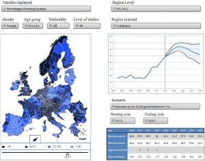
Concluding remarks
This article presents and to discuss an agent-based model of population dynamics for the European regions at NUTS 3 level. The technique of agent-based modelling has been chosen to allow including the concept of bounded rationality to the model and to combine demographic and economic data. The paper describes the latest novelties in this area of research, the process of data base creation as well as the model development and calibration. The database has been developed on the basis of the population census, and the input data is used then to obtain a model that helps to understand the dynamics of population and the relations between demography and economics. Each agent in the model passes sequentially through the five implemented modules: aging and deceases, education, pairing, labor market and migration.
In the first one. every agent computes a probability of death and there are determined the ones who decease. All members of population increase its age each year. There also has been taken into account the possibility of getting widowed or orphan. In the second one. individuals initiate their education, continue it or finish depending on the levels of studies previously received, age. gender and labor status. In the third part, the pairing process is analyzed.
Adult agents of one gender decide whether to get married, divorce or have children. In the following one, labor market characteristics are presented. Individuals have the choice of turning into inactive or starting looking for a job. The hiring and firing processes are also defined as well as the labor market demand in case of each of the regions. In the last one, the agents compute their satisfaction with their labor status and the probability of housing stress is taken into account as well. Also the decisions of staying or changing the place of living in the same region or for other one is included. At the same time, if individuals decide to change the region, the family also opts for changing their location.
For the purpose of model preparation, the one year iteration period was assumed. Parting from the data obtained from the reliable sources, the recalibrated model, jointly with the simulation, has been used to obtain the visualization for Spanish regions. Not only, the direct results for the next period have been obtained but also forecast of trends for the period between 2013 and 2021.
The novelty of this agent based model is the use of this technique in the studies of complex population dynamics phenomena. The applicability of this technique requires the adequate objects definition. In this paper, the following objects were defined: individuals as the agents that carry out the actions and populate the system, and families that are composed of individuals and have a possibility of migration. Notwithstanding, not only are objects individuals and families but also specific ones such as regions or space. The regional perspective assumed in the model allows the individuals to be located in the particular territory and then to analyze all consequences of changes in location or position. All regions include variables of aggregate outcomes and macroeconomic forecast. The other important object predefined in this version of population model is space. This object is represented by the matrix that includes the spatial distances between the centroid of every NUTS-3 region and cultural distances.
One of the most important features of this model is the preservation of the heterogeneity in the model. The heterogeneity was taken into account in the model by including the list of variables that specify the characteristics of the agents. At the same time we shall be aware of the benefits of the agent based modelling for population dynamics. Not only is the heterogeneity preserved but also the interactions and changes in individual’s behaviors depending on regional location are analyzed.
The population dynamics is not only about the demography and spatial location. It seems to be equally important to be able to carry out the full analysis of population dynamics is the impact of public policies and the position in the labor market of individuals. Those factors have a direct impact on individuals ’ and families ’ choices about their and other member of family ’ future. The definition of the labor market in the model presented hereby was elaborated assuming that it is composed by two different parts: a real labor supply integrated by individuals who decide if they will offer their workforce to the market or whether they prefer to be inactive, as well as the second one - an artificial labor demand-, computed adapting a set of standard macroeconomic rules. Its indirect aim is to contribute to the artificial labor market research mentioned in the introduction as well as to the general research on population dynamics modelling using the agent-based modelling.
The module presented by the authors is composed by the three methods: labor supply update, labor suitability update and labor market. The goal of this module has been to present the determinants of labor market movements but without doubts there exists also the other one, to test the methodology of research about the labor market shifts and their further consequences for the population.
The first method describes the process of getting retired and the results that change depending on the gender differences. This method is assumed to model the differences in individuals’ behavior and to preserve the heterogeneity in the behaviors defined in the system. The second one is used to update the labor demand. The update of valuation of individual’s power in the market has been included to represent faithfully the attractiveness of every individual for the labor demanders. As in the widely used models, a higher value increases the chances to be hired and decreases the probability of losing employment. In the third method, the complete labor market is defined by the inclusion of demand and supply sides.
Finally, the last module models the decision making of migration. There are two main determinants, the persistence of unemployment and the income variation across European regions. Individual decide their destination region according its characteristics and the spatial and cultural distance with their initial location. Immigration it is also taken into account.
This model makes possible to simulate and forecast the population dynamics of European regions in the period 2001-2021 and it explores how agent-based modelling can contribute to integrate demographics and economics to forecast accurately migration patterns as a result of labor and income differences between socioeconomic integrated areas as the European Union.
Notes
The authors are grateful to Alejandro Valbuena, IT engineer, for his kind collaboration validating the algorithms used in the SFE. This work has been conducted in the context of MOSIPS project (Modeling and Simulation of the Impact of public Policies on SMEs) of the EU 7th Framework Programme with Grant Agreement 288833.
Preprint submitted to ECCS’13 Satellite: Integrated Utility Services September 1, 2013